Adaptive QPE

Download this notebook - adaptive-qpe.ipynb

This example illustrates a possible implementation of a quantum algorithm in Guppy, showcasing the possible integration, usage and pitfalls of features including:

• Control flow

• Compile time expressions, especially for referencing global constants

The implemented algorithm is the basic adaptive random walk phase estimation algorithm found at arXiv:2208.04526 (Alg. 1 with sampling circuit from Fig. 1), with an example Hamiltonian and numbers taken from arXiv:2206.12950 (Section V.B).

Setup

We begin by specifying the example Hamiltonian in use, in this case \(H = 0.5 * Z\), in two variants:

1. The unitary oracle \(U(t) = R_Z[-0.5t]\) generated by the Hamiltonian, and

2. An eigenstate \(\ket{0}\) of the Hamiltonian.

Although this may seem redundant, we will need both for executing the algorithm.

from guppylang import guppy
from guppylang.std.quantum import qubit, crz


@guppy
def oracle(ctrl: qubit, q: qubit, t: float) -> None:
    """Applies a controlled e^-iπHt/2 gate for the example Hamiltonian H = 0.5 * Z."""
    crz(ctrl, q, angle(0.5 * t))


@guppy
def eigenstate() -> qubit:
    """Prepares eigenstate of the example Hamiltonian H = 0.5 * Z."""
    q = qubit()
    x(q)
    return q

Algorithm

The algorithm roughly performs the following steps on each iteration, which are outlined below:

1. Sample from a distribution generated by a circuit involving the eigenstate, an iteration-specific ancilla and the oracle (see Fig. 1 of arXiv:2208.04526).

2. Based on the outcome, step the phase estimate up or down by a fixed amount.

3. Decrease the step size by a fixed amount.

Following arXiv:2206.12950 (Fig. 4), we use 24 such iterations, and finally record the phase estimate using result.

import math
from guppylang.std.angles import angle
from guppylang.std.builtins import comptime, result
from guppylang.std.quantum import discard, measure, h, rz, x

sqrt_e = math.sqrt(math.e)
sqrt_e_div = math.sqrt((math.e - 1) / math.e)


@guppy
def main() -> None:
    # Pick initial estimate of phase mean and stdv
    # and prepare eigenstate
    mu, sigma = comptime(sqrt_e_div), 1 / comptime(sqrt_e)
    tgt = eigenstate()

    for _ in range(24):
        t = 1 / sigma

        # Sample from the phase estimate distribution
        aux = qubit()
        h(aux)
        rz(aux, angle((sigma - mu) * t))
        oracle(aux, tgt, t)
        h(aux)
        outcome = measure(aux)

        # Adjust estimate and step size
        if outcome:
            mu += sigma / comptime(sqrt_e)
        else:
            mu -= sigma / comptime(sqrt_e)
        sigma *= comptime(sqrt_e_div)

    discard(tgt)
    result("eigenvalue", 2 * mu)

main.check()

Note that the implementation uses comptime expressions to reference the constants sqrt_e and sqrt_e_div since they are defined outside the function annotated with @guppy.

One may ask why expressions involving sigma and these constants are not entirely wrapped in comptime. This uncovers a subtlety of such wrapping: comptime expressions are only evaluated once during compile time, and thus cannot react to changing variables such as sigma.

Testing and Evaluation

We test the implementation by creating an emulator and allocating the maximum number of qubits: One holding the eigenstate and one ancilla that will be reused. Running the emulator once yields an example result:

emulator = main.emulator(n_qubits=2).with_seed(2)
emulator.run()

EmulatorResult(results=[QsysShot(entries=[('eigenvalue', 2.3679925580437398)])])

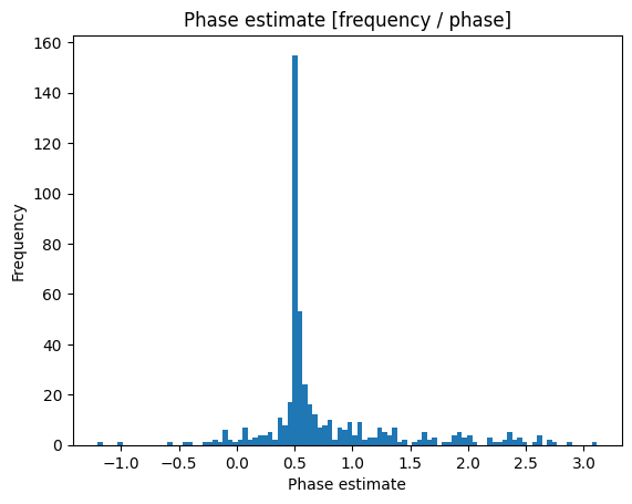
However, this is not guaranteed to be the actual phase of our example Hamiltonian, as it is only one example drawn from a distribution. We thus run a larger number of shots, extract the recorded phase from each and visualize them using matplotlib. Doing this reveals the expected phase of the Hamiltonian as the highest peak in the histogram.

import matplotlib.pyplot as plt
import matplotlib.ticker as ticker

shots = emulator.with_shots(500).run()

fig, ax = plt.subplots(1, 1)
ax.hist([shot.as_dict()["eigenvalue"] for shot in shots], bins=100)
ax.xaxis.set_major_locator(ticker.MultipleLocator(0.5))
ax.set_title("Phase estimate [frequency / phase]")
ax.set_xlabel("Phase estimate")
ax.set_ylabel("Frequency")
plt.show()