A simple Hubbard model simulation

The Hubbard model describes the motion and interactions of particles on a lattice and is often used to study strongly correlated materials. The extended Hubbard Hamiltonian included in InQuanto reads:

\[ H=\sum_{i} e_i c_i^{\dagger} c_i-t \sum_{<i,j>}-t' \sum_{<<i,j>>} c_i^{\dagger} c_j+U \sum_{i}n_{i\uparrow}n_{i\downarrow}+V \sum_{<i,j>} n_{i\uparrow} n_{j\downarrow}, \]

where \(e_i\) describes onsite energies, \(t\) (\(t'\)) denotes the hopping energy between (next) nearest neighboring sites, \(U\) stands for the onsite Hubbard interaction and \(V\) is the nearest neighbor Coulomb interaction.

Here we show an example of the ground state energy calculation for a small Hubbard square structure of \(2 \times 4\) sites. We start by building the Hamiltonian using the inquanto.express.DriverGeneralizedHubbard2D. More information on how to use this driver can be found here.

from inquanto.express import DriverGeneralizedHubbard2D
from inquanto.ansatzes import SiteLabeling2D

e, t, u, v, nx, ny = (0.0, -1.0, 4.0, 0.0, 2, 4)
labels = SiteLabeling2D.snake
hubbard_driver = DriverGeneralizedHubbard2D(
    e=e, u=u, t=t, v=v, n_x=nx, n_y=ny, site_labeling=labels, pbc=False
)

ham, f_space, f_state = hubbard_driver.get_system()
print('\nSnake Hamiltonian:\n', ham.df())

Snake Hamiltonian:
     Coefficient                 Term         Coefficient type
0          -1.0              F0^ F2   <class 'numpy.float64'>
1          -1.0              F0^ F6   <class 'numpy.float64'>
2           4.0      F1^ F0^ F0  F1   <class 'numpy.float64'>
3          -1.0              F1^ F3   <class 'numpy.float64'>
4          -1.0              F1^ F7   <class 'numpy.float64'>
5          -1.0              F2^ F0   <class 'numpy.float64'>
6          -1.0              F2^ F4   <class 'numpy.float64'>
7          -1.0              F3^ F1   <class 'numpy.float64'>
8           4.0      F3^ F2^ F2  F3   <class 'numpy.float64'>
9          -1.0              F3^ F5   <class 'numpy.float64'>
10         -1.0              F4^ F2   <class 'numpy.float64'>
11         -1.0              F4^ F6   <class 'numpy.float64'>
12         -1.0             F4^ F10   <class 'numpy.float64'>
13         -1.0              F5^ F3   <class 'numpy.float64'>
14          4.0      F5^ F4^ F4  F5   <class 'numpy.float64'>
15         -1.0              F5^ F7   <class 'numpy.float64'>
16         -1.0             F5^ F11   <class 'numpy.float64'>
17         -1.0              F6^ F0   <class 'numpy.float64'>
18         -1.0              F6^ F4   <class 'numpy.float64'>
19         -1.0              F6^ F8   <class 'numpy.float64'>
20         -1.0              F7^ F1   <class 'numpy.float64'>
21         -1.0              F7^ F5   <class 'numpy.float64'>
22          4.0      F7^ F6^ F6  F7   <class 'numpy.float64'>
23         -1.0              F7^ F9   <class 'numpy.float64'>
24         -1.0              F8^ F6   <class 'numpy.float64'>
25         -1.0             F8^ F10   <class 'numpy.float64'>
26         -1.0             F8^ F14   <class 'numpy.float64'>
27         -1.0              F9^ F7   <class 'numpy.float64'>
28          4.0      F9^ F8^ F8  F9   <class 'numpy.float64'>
29         -1.0             F9^ F11   <class 'numpy.float64'>
30         -1.0             F9^ F15   <class 'numpy.float64'>
31         -1.0             F10^ F4   <class 'numpy.float64'>
32         -1.0             F10^ F8   <class 'numpy.float64'>
33         -1.0            F10^ F12   <class 'numpy.float64'>
34         -1.0             F11^ F5   <class 'numpy.float64'>
35         -1.0             F11^ F9   <class 'numpy.float64'>
36          4.0  F11^ F10^ F10  F11   <class 'numpy.float64'>
37         -1.0            F11^ F13   <class 'numpy.float64'>
38         -1.0            F12^ F10   <class 'numpy.float64'>
39         -1.0            F12^ F14   <class 'numpy.float64'>
40         -1.0            F13^ F11   <class 'numpy.float64'>
41          4.0  F13^ F12^ F12  F13   <class 'numpy.float64'>
42         -1.0            F13^ F15   <class 'numpy.float64'>
43         -1.0             F14^ F8   <class 'numpy.float64'>
44         -1.0            F14^ F12   <class 'numpy.float64'>
45         -1.0             F15^ F9   <class 'numpy.float64'>
46         -1.0            F15^ F13   <class 'numpy.float64'>
47          4.0  F15^ F14^ F14  F15   <class 'numpy.float64'>

Hamiltonian variational ansatz

Quantum simulations of Hubbard systems often employ the VQE framework to find the ground state energy of the problem. This involves proposing an initial state with free parameters. These parameters are classically optimized in a loop that is guided by the quantum computed energy of the system. The success of this technique depends strongly on the selection of an efficient ansatz that still captures the problem’s features [Cade et al.].

A popular ansatz choice is the Hamiltonian Variational Ansatz (HVA), which takes inspiration from the adiabatic theorem. It mimics the adiabatic evolution of the state under the Hubbard Hamiltonian by applying a sequence of rotations with variational parameters instead of fixed time intervals [Wecker et al.]. More details on constructing a general HVA can be found here.

Below we show how a simple HVA is constructed in InQuanto for the Hubbard model on a square lattice. First, the Hubbard Hamiltonian for a square lattice is split into commuting parts [Cade et al.]:

\[ H_e=\sum_{i}e_i c_i^{\dagger}c_i \]

\[ H_U=U\sum_{i} n_{i\uparrow}n_{i\downarrow} \]

\[ H_V=V\sum_{<i,j>\sigma} n_{i\sigma}n_{j\sigma} \]

\[ H_{h_e}=-t_{h_e}\sum_{<i,j> \text{horiz even}} c_i^{\dagger}c_j+h.c. \]

\[ H_{h_o}=-t_{h_o}\sum_{<i,j> \text{horiz odd}} c_i^{\dagger}c_j+h.c. \]

\[ H_{v_e}=-t_{v_e} \sum_{<i,j> \text{vert even}} c_i^{\dagger}c_j+h.c. \]

\[ H_{v_o}=-t_{v_o} \sum_{<i,j> \text{vert odd}} c_i^{\dagger}c_j+h.c., \]

\[ H_{next}=-t' \sum_{<<i,j>>} c_i^{\dagger}c_j+h.c., \]

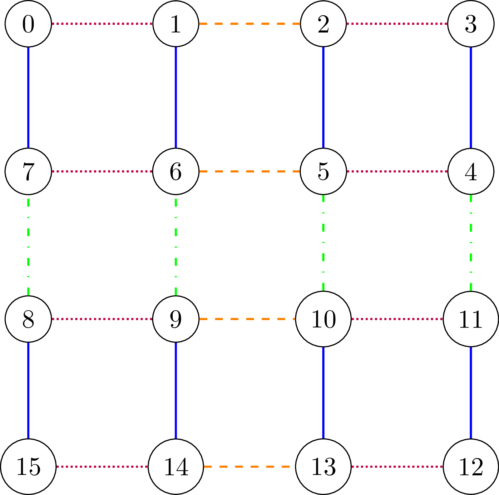
where \(H_e\) is the onsite term, \(H_U\) is the Hubbard U term, \(H_{h_e}\) is the horizontal hopping term for even (red dotted in the figure above) and \(H_{h_o}\) for odd (orange dashed in the figure above) and \(H_{v_e}\) and \(H_{v_o}\) are the vertical hopping terms for even (blue solid in the figure above) and odd rows (green dash-dotted in the figure above), and \(H_{next}\) is the next nearest neighbor hopping (not shown in the figure for clarity). Not all of these terms will be present for a small structure, but they have been listed and shown here for generality. Each term is multiplied by a variational parameter and used in a unitary rotation. The sequence of all rotations by all terms is then repeated \(s\) times for an \(s\)-layer HVA.

\[ \Psi_{HVA}=\prod_{k=1}^s e^{-i\phi_{0k}H_V} e^{-i\phi_{1k}H_U} e^{-i\phi_{2k}H_ho} e^{-i\phi_{3k}H_he} e^{-i\phi_{4k}H_{ve}} e^{-i\phi_{5k}H_{vo}} e^{-i\phi_{k}H_{next}} |\psi_i\rangle. \]

The inquanto.express.HamiltonianVariationalAnsatzHubbard has \(m \cdot s\) variational parameters, one for each Hamiltonian term in each layer, and \(m\) denotes distinct term types in the Hamiltonian.

We show an example of how to use HVA for the Hubbard model solution in the next section. Examples of using HVA for solving chemistry problems can be found here.

Slater determinant state preparation

Part of the task of preparing a good HVA involves the choice of an appropriate initial reference state that the ansatz builds upon. This choice corresponds to selecting a specific phase characterized by spin or particle number, which is expected to describe the solution of the Hubbard Hamiltonian.

One common way to build a reference state is to arrange \(N=N_{\uparrow}+N_{\downarrow}\) particles on the first \(N\) sites of the lattice, with alternating spins, producing an antiferromagnetic state [Wecker et al.]. This type of state is the default output by the get_system() method used above.

Another good choice of a reference state is to initialize the system in the eigenstate of the non-interacting part of the Hamiltonian, i.e. a single Slater determinant (SD) [Wecker et al.]. The ansatz will then account account for the other (interacting) terms. Coefficients for such a SD state can be obtained by diagonalizing a tight-binding Hamiltonian or a mean-field problem first. A SD reference state can be built with InQuanto by providing a unitary matrix rotation [Jiang et al.], [Kivlichan et al.] using inquanto.ansatzes.RealGeneralizedBasisRotationAnsatz, inquanto.ansatzes.RealRestrictedBasisRotationAnsatz and inquanto.ansatzes.RealUnrestrictedBasisRotationAnsatz.

Solving the Hubbard model with VQE

Here we will put all the above components together to build a Hubbard model simulation for the \(2 \times 4\) structure mentioned at the beginning, using the VQE algorithm.

We start with building a SD reference state for the HVA ansatz. A reference state is built from the rotation matrix corresponding to the eigenstates of the hopping matrix. The hopping matrix is obtained from the InQuanto Hubbard driver.

from inquanto.mappings import QubitMappingJordanWigner
from inquanto.ansatzes import RealUnrestrictedBasisRotationAnsatz
import numpy as np

# Get the hopping matrix from the driver (without the Hubbard U term)
hopping_matrix, _ = hubbard_driver.get_one_two_body_terms()
n_sites = nx * ny

# Define fermion to qubit mapping and map the Hamiltonian
mapping = QubitMappingJordanWigner()
qubit_op = mapping.operator_map(ham)

# Diagonalise the non-interacting problem
eigvals, eigvecs = np.linalg.eigh(hopping_matrix.todense())

# Set up the number of particles for one spin and prepare a state with this number
n_el_one_spin = 4
reference_state = [1] * 2 * n_el_one_spin + [0] * (n_sites - n_el_one_spin) * 2

# Rotate the reference state to the basis diagonalising the non-interacting problem
rotation_driver = RealUnrestrictedBasisRotationAnsatz(reference_state)
rotation_params = rotation_driver.ansatz_parameters_from_unitary(eigvecs, eigvecs)
slater_det_circuit = rotation_driver.get_circuit(rotation_params)

We then define the HVA with the SD reference state and a given number of layers.

from pytket.extensions.qiskit import AerStateBackend
from inquanto.ansatzes import HamiltonianVariationalAnsatzHubbard

# Define the HVA ansatz. The Slater determinant circuit needs to be compiled
backend = AerStateBackend()
compiled_circuit = backend.get_compiled_circuit(slater_det_circuit)


# define the ansatz and starting parameters for a Hubbard model VQE calculation
init_params = {"sym0_l0": 0.9481931804543265, "sym0_l1": 1.0382884839454627, "sym0_l2": -0.924132119830008,
                  "sym1_l0": 1.1082735281121958, "sym1_l1": 2.022564270774505, "sym1_l2": -0.08425721713315654,
                  "sym2_l0": -0.6123566351342871, "sym2_l1": 0.7032504509643882, "sym2_l2": 0.9633159435158412,
                  "sym3_l0": -0.6556278859648624, "sym3_l1": -1.010560960893456, "sym3_l2": -0.12415371369806133}

n_layer = 3  # number of layers in the ansatz used for accuracy adjustment
ansatz = HamiltonianVariationalAnsatzHubbard(compiled_circuit, lat_dims=[nx, ny],
                                             hamiltonian_operator=ham,
                                             step_number=n_layer, site_labeling=labels)

We then build a VQE algorithm and run it.

from inquanto.algorithms import AlgorithmVQE
from inquanto.computables import ExpectationValue, ExpectationValueDerivative
from inquanto.minimizers import MinimizerScipy
from inquanto.protocols import SparseStatevectorProtocol

# build the VQE algorithm
expectation_value = ExpectationValue(ansatz, qubit_op)
derivative = ExpectationValueDerivative(ansatz, qubit_op, ansatz.state_symbols.as_set())
vqe = AlgorithmVQE(
    objective_expression=expectation_value,
    minimizer=MinimizerScipy(),
    gradient_expression=derivative,
    initial_parameters=init_params,
)

# Define circuit protocols
protocol_objective = SparseStatevectorProtocol(backend)
protocol_gradient = SparseStatevectorProtocol(backend)
vqe.build(
    protocol_objective=protocol_objective,
    protocol_gradient=protocol_gradient
)

# Run the VQE algorithm
vqe.run()

# print final VQE energy
print("VQE Energy:    ", vqe.final_value)
print("VQE Parameters:", vqe.final_parameters)

# TIMER BLOCK-0 BEGINS AT 2026-04-23 14:00:52.515487
# TIMER BLOCK-0 ENDS - DURATION (s): 22.0879024 [0:00:22.087902]
VQE Energy:     -4.268977767009267
VQE Parameters: {sym0_l0: np.float64(0.9481971507635327), sym0_l1: np.float64(1.0382907258804654), sym0_l2: np.float64(-0.9241355898527304), sym1_l0: np.float64(1.108270510078506), sym1_l1: np.float64(2.0225629344784775), sym1_l2: np.float64(-0.08426166333799054), sym2_l0: np.float64(-0.6123580126341529), sym2_l1: np.float64(0.703253523575341), sym2_l2: np.float64(0.9633103448578884), sym3_l0: np.float64(-0.6556297039663058), sym3_l1: np.float64(-1.010559715335178), sym3_l2: np.float64(-0.12415347884908916)}

The form of the HVA ansatz used here is not sufficiently complex to reproduce the exact GS energy, equal to \(E_{GS}=-5.0\). In order to obtain accurate energy, likely \(n_{layer}=10\) would be needed. However, the wavefunction obtained from this algorithm already gives a good representation of the ground state.

Measuring the ground state spin correlations

Often, the goal of solving the Hubbard model on a quantum computer is learning more about the nature of its ground state in various areas of the phase space. This can be achieved by e.g. tracking charge and spin observables as the model parameters change. Expectation values of charge and spin operators can be obtained using InQuanto, just like the energy expectation values we needed in each iteration of VQE.

Spin correlation is given by [Stanisic et al.]:

\(C(i,j) = \langle S_z^i S_z^j \rangle - \langle S_z^i\rangle \langle S_z^j\rangle\),

where \(S_z^i\) is the \(z\) projection of the spin operator on site \(i\).

Here we show how to produce a spin correlation matrix for the ground state that we obtained from VQE using InQuanto. The SpinCorrelationComputable relies on the fermion space object f_space generated by the Hubbard driver to produce the necessary spin operators.

from inquanto.computables.composite import SpinCorrelationComputable

# define the spin correlation computable
spin_corr_comp = SpinCorrelationComputable(f_space, ansatz, mapping)
print(f"spin correlation computable: {spin_corr_comp}")

spin correlation computable: <inquanto.computables.composite._spin_correlation.SpinCorrelationComputable object at 0x76fbc5c06330>

We now evaluate the SpinCorrelationComputable and plot the results.

from matplotlib import pyplot as plt
# evaluator driver
evaluator = protocol_objective.get_evaluator(vqe.final_parameters)
# evaluate spin correlation
spin_corr_exp_val = spin_corr_comp.evaluate(evaluator=evaluator)
# extract the spin correlation matrix to plot
spin_corr_mat = np.real(spin_corr_exp_val.data)

# plot results
plt.figure()
plt.imshow(spin_corr_mat)
plt.colorbar()
plt.title(f"Spin correlation for 2x4 lattice")
plt.show()

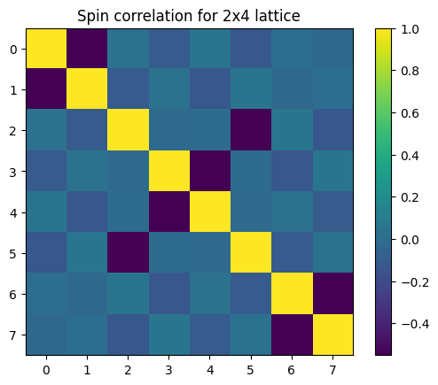
The result we obtain is a 8x8 matrix, with rows and columns corresponding to all the sites of the lattice structure. This is in agreement with [Stanisic et al.] (Fig. 6c.).