Demonstration of Quantum Error-Corrected Quantum Phase Estimation

This knowledge article is based on version one of the arxiv pre-print of Quantum Error-Corrected Computation of Molecular Energies by Yamamoto et al. (arXiv:2505.09133v1), submitted on 14 May 2025.

Computational chemistry holds promise as an application for quantum computing, holding the potential for an exponential speed-up over classical methods and ultimately providing access to solutions for problems that are classically intractable.

Several quantum algorithms have been developed and adapted for the electronic structure problem. Quantum phase estimation (QPE) has emerged as an effective algorithm for calculating molecular energies on quantum computers. However, there is still progress to be made to achieve quantum advantage over classical computers. Although physical qubit counts and gate operation fidelities continue to rise and algorithmic developments move along steadily, even the most resource efficient QPE circuits accumulate infeasible physical errors on today’s noisy hardware.

To achieve a scalable implementation of QPE, quantum error correction (QEC) techniques must be applied. A team of Quantinuum researchers did exactly that, running partially fault tolerant (PFT) QPE experiments on System Model H2 to estimate the ground state energy of H₂ in the STO-3G basis. The error in the energy estimate compared to the full configuration interaction energy was 0.018 hartree. Furthermore, we ran numerical simulations on the H2-Emulator, determining that memory error was the dominant source of noise in this experiment.

This knowledge first summarizes the arxiv pre-print, Quantum Error-Corrected Computation of Molecular Energies, by Yamamoto et al. (arXiv:2505.09133v1). Then, it demonstrates how users can recreate and extend upon some of the experiments with InQuanto. Users are able to investigate different Hamiltonians and choose the QEC techniques applied at various steps in the construction of the logical circuits. This is a minimal implementation of error correction as applied to chemical computations. More extensive tools related to error correction are available here.

Quantum Phase Estimation

We chose to use the information theory flavor of QPE for this experiment. As an iterative form of QPE, information theory QPE trades a shallower circuit, only requiring a single controlled unitary operation and a single ancilla qubit, for a larger number of shots. You can read more about using information theory QPE in InQuanto here. The figure below depicts the QPE circuit used in this experiment at the logical level.

The circuit has four key components:

1. Preparation of ancilla (\(\ket{+}\)) and system (\(\ket{\Phi}\)) input states

2. Application of \(U^k\) on the system register, conditioned on the ancilla qubit

3. Application of the phase-shift gate, Rz(\(\beta\))

4. Measurement of the ancilla qubit in the \(X\) basis

In our experiments the trial input state (\(\ket{\Phi}\)) used was the qubit-encoded Hartree-Fock state, and the unitary operator \(U\) encoded the real time evolution under the Hamiltonian of the H₂ molecule in minimal basis and at equilibrium geometry.

In the implementation of information theory QPE used here, the circuit was executed multiple times, each with random values of \(k\) and \(\beta\). These measurement samples (shots) were post-processed to build distribution of phases. Then, the desired phase was estimated by the maximum likelihood of this distribution. The accuracy of this technique depends on several parameters; the maximum value of \(k\) (here set to 12), the number of shots run, and the overlap of the input state with the ground state.

While this QPE circuit requires few qubits, the number of gates required to implement \(cntrl-U^k\) naïvely on today’s noisy quantum hardware would require unrealistic physical error rates. Therefore, QEC techniques were used to design the circuits to be executed on System Model H2, suppressing the inevitable accumulation of errors. Fault tolerant (FT) design principles were used to attempt to minimize the effect of errors introduced by the QEC procedures themselves.

Quantum Error Correction

Quantum Error Correction codes necessarily encode a smaller number of logical qubits into a larger number of physical qubits. Encoding logical qubits allows degrees of freedom at the physical level to be measured during execution of the circuit without disturbing the logical information. We then aim to apply corrective operations based on these measurements to stop physical errors from accumulating into logical errors. These corrections can be applied during runtime or in postprocessing. However, QEC comes with a significant resource overhead.

As mentioned, multiple physical qubits are required to produce a logical qubit. Logical qubits then necessitate logical operations implemented using several physical gate operations. In this work, the \([[7, 1, 3]]\) color code (Steane code) was implemented, compiling the circuits into the Clifford + Rz(\(\theta\)) gate set. A \([[k, n, d]]\) QEC code requires \(k\) (7) physical qubits to encode \(n\) (1) logical qubit to a distance \(d\) (3). The distance of a code relates to the weight (number of qubits the logical operators act on) of physical errors that a code can correct, given by \(\lfloor d/2 \rfloor\). With \(d/2 = 1.5\), this color code can correct a physical single qubit error.

In practice, building and executing a fully FT circuit results in a significant resource overhead. Therefore, partially fault tolerant setups that aim to gain some of the benefit of QEC while minimizing the added resource overhead have been developed. For the current era of devices, these may give increased performance compared to full FT setups. In this experiment, we designed three QPE circuit setups with varying levels of fault-tolerance: the simulation setup (Sim), the experimental setup (Exp), and the control setup (Con).

Partially fault tolerant setups

The Sim setup involved FT preparation of the \(\ket{+}\) state of the ancilla. The QPE input state \(\ket{\Phi}\) was also prepared fault tolerantly using error detection. Here, a quantum error detection (QED) gadget serves to detect faults. If a fault is detected, the state is discarded and then preparation is repeated. The Sim controlled unitary gate included error-correcting QEC gadgets on both the ancilla and system registers. Then, the phase shift rotation Rz(\(\beta\)) was applied to the ancilla register in an identical manner to the input state, with an error detection component. Finally, measurement in the Pauli \(X\) basis was implemented fault tolerantly. Of the three setups, Sim implemented the most QEC gadgets, consequently requiring the largest circuit resources: 22 physical qubits, up to 2185 physical two-qubit gates, and 760 mid-circuit measurements.

The Exp setup included non-FT \(\ket{+}\) and input state \(\ket{\Phi}\) preparation (without QED). QEC gadgets were only applied to the ancilla register during the application of the controlled unitary. The phase-shift rotation gate Rz(\(\beta\)) was applied without error detection and finally, measurement in the Pauli-X basis was implemented fault-tolerantly. The last setup, Con, was identical to the Exp setup , but without the QEC gadget on the ancilla register of the controlled unitary operation.

Results from System Model H2

The Exp circuit was executed on System Model H2 for a maximum of 2300 shots resulting in a ground state energy estimate of H₂ in the STO-3G basis. The difference between the experimentally estimated energy (\(E_{Exp}\)) and the classically calculated FCI energy (\(E_{FCI}\)) was \(E_{Exp}-E_{FCI} = 0.018~hartree\). While this is not within the bounds of chemical precision (\(\sim~0.0016~hartree\)), it is an important milestone on the way to that goalpost. We also took care to confirm that the QEC gadgets applied in the Exp setup were effective in suppressing errors. By comparing the circuit infidelity for various values of \(k\) (power of \(U\)) between the Exp and Con setups run on the H2-Emulator, we showed that at large values of \(k\) (12) the Exp setup had a better fidelity than Con. We also observed that the Con setup had a relatively small infidelity at small \(k\), indicating that the FT \(X\) basis measurement worked well to suppress the measurement error for shallower circuits. Numerical simulations described in the second part of the paper indicate where improvements can be made to help reach the chemical precision goalposts.

With the ability to select and adjust the sources of noise within the H2-Emulator, we were able to determine the dominant noise source for the Sim setup through numerical simulations. Memory error, which arises due to long idling and ion-transport times, was determined the dominant source of noise. These idling and ion-transport times were longest for the Sim setup due to the complex conditional operations required to apply the QEC techniques. Circuit techniques such as dynamical decoupling can be used to reduce the total memory error accumulated during circuit execution. The application of higher distance QEC codes - those that allow the correction of multi-qubit errors of higher weight - may also suppress not only the memory error, but all other forms of error, depending on the distance of the code.

Using software and hardware developed in-house, a multi-disciplinary team of scientists and engineers performed a world first in quantum error-corrected quantum phase estimation for the purpose of determining molecular energies. This work lays an important stepping stone, paving the way to scalable and FT calculations of molecular energies on quantum computers. Following is a demonstration of quantum error correction applied to information theory phase estimation for the estimation of ground state energies.

Demonstration with InQuanto

We replicate the approach of Yamamoto et al. (arXiv:2505.09133v1) using InQuanto to change the Hamiltonian of interest. The core settings rely on the creation of a ChemData instance. The target Hamiltonian, along with other parameters of interest are specified in this object.

• CZ, CX, and CI are the weights for the corresponding Pauli gates that comprise the single qubit Hamiltonian.

• DELTA_T is the time step

• MAX_BITS is the number of bits for rounding rotation angles

• FCI_ENERGY is the calculated FCI energy of H2 in the STO-3G basis

• APPROX_ENERGY is the FCI energy + trotter error (APPROX_PHASE/DELTA_T)

• ANSATZ_PARAM are the parameter values for the ansatz

• APPROX_PHASE is the eighenphase of the Trotterized Hamiltonian

• HF_STATE is the occupation number representation of the input HF state

The specific settings used in the paper can be obtained with the inquanto.qec_qpe_chem.experiment.H2_DATA configuration:

from inquanto.experiments.qec_qpe_chem.experiment import ChemData
from inquanto.experiments.qec_qpe_chem.experiment import H2_DATA
print(H2_DATA)

import warnings
warnings.filterwarnings('ignore')

ChemData(CZ=0.7960489286466914, CX=-0.1809233927385484, CI=-0.3209561440881913, DELTA_T=0.3140508999066516, MAX_BITS=5, FCI_ENERGY=-1.13730605, APPROX_ENERGY=-1.13629792, ANSATZ_PARAM=[-0.08728706, -0.25], APPROX_PHASE=-0.3568553843380564, HF_STATE=1)

An instance of ChemData may be constructed manually - note that the APPROX_PHASE and HF_STATE parameters are determined automatically based on the provided data:

chem_data_manual = ChemData(CZ=1.,
                            CX=0.,
                            CI=0.,
                            DELTA_T=1.,
                            MAX_BITS=5,
                            FCI_ENERGY=-1.,
                            APPROX_ENERGY=-1.,
                            ANSATZ_PARAM=[0.,0.])
print(chem_data_manual)

ChemData(CZ=1.0, CX=0.0, CI=0.0, DELTA_T=1.0, MAX_BITS=5, FCI_ENERGY=-1.0, APPROX_ENERGY=-1.0, ANSATZ_PARAM=[0.0, 0.0], APPROX_PHASE=-1.0, HF_STATE=1)

The specification of quantities which are exponentially costly to classically precompute are optional (FCI_ENERGY, APPROX_ENERGY, ANSATZ_PARAM, APPROX_PHASE). However, not providing these quantities will restrict the available functionality, particularly the ability to benchmark the effectiveness of the QEC components.

chem_data_manual_minimal = ChemData(CZ=1.,
                            CX=0.,
                            CI=0.,
                            DELTA_T=1.)
print(chem_data_manual)

ChemData(CZ=1.0, CX=0.0, CI=0.0, DELTA_T=1.0, MAX_BITS=5, FCI_ENERGY=-1.0, APPROX_ENERGY=-1.0, ANSATZ_PARAM=[0.0, 0.0], APPROX_PHASE=-1.0, HF_STATE=1)

Defining the system of interest

The ChemData object may be generated from an InQuanto QubitOperator, allowing for the use of different Hamiltonians while replicating the experiment described in Yamamoto et al. We are still restricted to the use of 1-qubit Hamiltonians, but this nevertheless allows for some experimentation: for example, we could attempt the experiment using a Hamiltonian corresponding to the molecule at a slightly stretched bondlength (0.735 Angstrom), rather than the equilibrium geometry used in the paper.

In the cell below, we first use InQuanto to read the molecular data from the express module, generate the fermionic Hamiltonian, map the state and Hamiltonian to qubits, and then taper the resulting qubit Hamiltonian down to a single qubit.

from inquanto.symmetry import TapererZ2
from inquanto.spaces import QubitSpace
from inquanto.mappings import QubitMappingJordanWigner
from inquanto.express import load_h5

data = load_h5("h2_sto3g_long.h5",as_tuple=True)
fermionic_hamiltonian = data.hamiltonian_operator.to_FermionOperator()
fermionic_hf_state = data.hf_state

qubit_hamiltonian = QubitMappingJordanWigner.operator_map(fermionic_hamiltonian)
qubit_hf_state = QubitMappingJordanWigner.state_map(fermionic_hf_state)
symmetry_operators = QubitSpace(4).symmetry_operators_z2(qubit_hamiltonian)
symmetry_sectors = [x.symmetry_sector(qubit_hf_state) for x in symmetry_operators]
taperer = TapererZ2(symmetry_operators,symmetry_sectors)

tapered_operator = taperer.tapered_operator(qubit_hamiltonian)
print(tapered_operator)

(-0.32112414706764547, I0), (0.7958748496863586, Z0), (0.18093119978423144, X0)

We have two primary methods for generating ChemData objects from a given Hamiltonian. The first is ChemData.from_qubit_operator. This optionally allows specification of the costly parameters (FCI_ENERGY etc.); however, here we will leave them unspecified. In this case, DELTA_T is inferred so as to result in a circuit with a \(Z\) rotation corresponding to a single T gate, as described in the paper.

chemdata_minimal = ChemData.from_qubit_operator(tapered_operator)
print(chemdata_minimal)

ChemData(CZ=0.7958748496863586, CX=0.18093119978423144, CI=-0.32112414706764547, DELTA_T=0.31411973892443135, MAX_BITS=5, FCI_ENERGY=None, APPROX_ENERGY=None, ANSATZ_PARAM=None, APPROX_PHASE=None, HF_STATE=1)

The alternative is to use the ChemData.from_qubit_operator_automated method, which will automatically calculate all extra parameters in accordance with the method described in the paper. This approach is not scalable, but allows for the use of the “benchmarking mode” as discussed below.

chemdata_full = ChemData.from_qubit_operator_automated(tapered_operator)
print(chemdata_full)

ChemData(CZ=0.7958748496863586, CX=0.18093119978423144, CI=-0.32112414706764547, DELTA_T=0.31411973892443135, MAX_BITS=5, FCI_ENERGY=-1.1373060357533997, APPROX_ENERGY=-1.1329833131949456, ANSATZ_PARAM=array([ 0.071, -0.   ]), APPROX_PHASE=-0.3558924225465335, HF_STATE=1)

Executing experiments

Having generated chemdata_full, we can now replicate the procedures described in the publication with our new Hamiltonian. We start with the “benchmarking mode”. First we build the logical QPE circuits (there is one circuit for each value of \(k\) provided). Here we need to specify i) the powers of the Hamiltonian that we want to apply (k_list), ii) whether or not we wish to implement the \(Rz(\beta)\) in a partially fault tolerant manner (pft_rz) using error detection, and iii) the qec_level. The qec_level values corresponds to the control (Con, 0), experimental (Exp, 1), and simulation (Sim, 2) setups previously described.

from inquanto.experiments.qec_qpe_chem.experiment import build_benchmark_circuits
from inquanto.experiments.qec_qpe_chem.encode import encode, EncodeOptions, RzMode
from pytket.extensions.quantinuum import (
    QuantinuumBackend,
    QuantinuumAPIOffline,
)
from inquanto.experiments.qec_qpe_chem.encode import InterpretOptions, ReadoutMode, interpret
from inquanto.experiments.qec_qpe_chem.experiment import process_benchmark_results
from pytket.circuit.display import render_circuit_jupyter


k_list = [1, 2, 3, 4]
pft_rz =  False
qec_level = 0

logical_circuits = build_benchmark_circuits(chemdata_full,
    k_list=k_list,
    pft_rz=pft_rz,
    qec_level=qec_level,
)

render_circuit_jupyter(logical_circuits[0])

The next step is to encode the logical circuits using the \([[7, 1, 3]]\) color (Steane) code. EncodeOptions allows us to specify how components of the logical circuit are encoded. rz_mode determines how the \(Rz(\beta)\) gate is logically encoded. The RzMode object gives us four options to choose from, outlined in Table 1. of the paper (in order of increasing overhead):

• DIRECT implements the operation directly in addition to a QED component (\(\overline{R}^{D, QED}_Z(\theta)\))

• BIN_FRAC_NON_FT employs the recursive gate teleportation technique with non-FT state preparation and measurement

• BIN_FRAC_MEAS_FT improves on BIN_FRAC_NON_FT with FT measurement (\(\overline{R}^{RGT}_Z(\theta)\))

• BIN_FRAC_PART_FT improves on BIN_FRAC_MEAS_FT by implementing QED on the state preparation (\(\overline{R}^{RGT, QED}_Z(\theta)\))

We can also enable FT state preparation of the input state register (ft_prep) and the ancilla register (ft_prep_synd). However, to keep this notebook computationally tractable, we have disabled them here.

encoded_circuits = [
    encode(
        circ,
        options=EncodeOptions(
            rz_mode=RzMode.DIRECT,
            ft_prep=False,
            ft_prep_synd=False,
        )
    ) for circ in logical_circuits
]

render_circuit_jupyter(encoded_circuits[0])

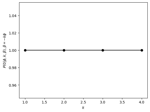
The encoded circuits can then be compiled and executed on a backend, here we use a local noiseless emulator of System Model H2-1. The physical results are interpreted with knowledge of what QEC and QED components were used to create the encoded circuits, providing logical results. These are then processed to return the probabilities of a successful, error corrected outcome (0). While the noiseless results give the expected 100% probability, swapping H2-1LE for a noisy Quantinuum backend produces the expected exponential decay in success probability with increasing k.

Users can experiment here with the different readout modes. Each mode applies a level of fault tolerance to the measurement outcomes, from the non-FT ReadoutMode.Raw to the FT ReadoutMode.Correct.

backend = QuantinuumBackend(
    device_name="H2-1LE",
    api_handler=QuantinuumAPIOffline(),
) # Noiseless local emulator of System Mo

compiled_circuits = backend.get_compiled_circuits(
    encoded_circuits,
    optimisation_level=0,
)
N_SHOTS = 10

encoded_results = backend.run_circuits(
    compiled_circuits,
    n_shots=N_SHOTS,
)
logical_results = [
    interpret(
        result,
        options=InterpretOptions(
            readout_mode=ReadoutMode.Correct, # Perform error correction on the measurements
            # readout_mode=ReadoutMode.Detect, # Error detect on the measurements
            # readout_mode=ReadoutMode.Raw, # Interpret raw measurement outcomes
        ),
    ) for result in encoded_results
]
benchmark_results = process_benchmark_results(logical_results)

import matplotlib.pyplot as plt

plt.plot(k_list, benchmark_results.p0, "k-o")
plt.ylabel(r"$P(0|\phi, k, \beta), \beta =-k\phi$")
#Probability to measure 0 as a function of k when beta is set to reflect the true phase
plt.xlabel(r"$k$");

Note that attempting to use this benchmark process with a partially-filled ChemData object will result in an error:

# Uncomment to see example below
# logical_circuits = build_benchmark_circuits(chemdata_minimal,
#     k_list=k_list,
#     pft_rz=pft_rz,
#     qec_level=qec_level,
# )

However, we can use the partially-filled ChemData object to compute the energy of the molecule using the information theory QPE. Notice that we now generate a list of random values for \(k\) and \(\beta\), eventually building 25 logical circuits with combinations of these.

from inquanto.experiments.qec_qpe_chem.algorithm import get_ms, bayesian_update, bootstrap_sampling
from inquanto.experiments.qec_qpe_chem.experiment import build_iqpe_circuits
import numpy as np

k_max = 5
n_samples = 25
k_list = np.random.randint(1, k_max+1, size=n_samples).tolist()
beta_list = (1 - 2 * np.random.random(size=n_samples)).tolist()
logical_circuits = build_iqpe_circuits(chemdata_minimal,
    k_list=k_list,
    beta_list=beta_list,
    pft_rz=False,
    qec_level=0,
)

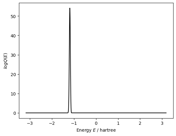
The logical circuits are then encoded, compiled, and executed as before. The measurement results can then be post-processed to extract a distribution over phases (Below, \(Q(\phi)\)). This distribution is transformed into \(Q(E)\), the distribution of energies, peaked around an approximation to the eigenvalue of the Hamiltonian. The accuracy of this estimate depends on \(k_{max}\), the number of shots run, and the population of the eigenstate in the input state. The final figure that is output from the cell below shows the distribution of energy eigenvalues, with it’s peak at the most likely estimate of the ground state energy.

encoded_circuits = [
    encode(
        circ,
        options=EncodeOptions(
            rz_mode=RzMode.DIRECT,
        )
    ) for circ in logical_circuits
]

backend = QuantinuumBackend(
    device_name="H2-1LE",
    api_handler=QuantinuumAPIOffline(),
)
compiled_circuits = backend.get_compiled_circuits(
    encoded_circuits,
    optimisation_level=0,
)
N_SHOTS = 5

encoded_results = backend.run_circuits(
    compiled_circuits,
    n_shots=N_SHOTS,
)

logical_results = [
    interpret(
        result,
        options=InterpretOptions(
            readout_mode=ReadoutMode.Raw, # Use the readout as it is
        ),
    ) for result in encoded_results
]


ks, betas, ms = get_ms(k_list, beta_list, logical_results)

# Prepare the uniform prior distribution.
n_grid_points = 2 ** 10
phi = np.linspace(-1, 1, n_grid_points+1)[:-1]
prior = np.ones_like(phi)

mu, sigma = bootstrap_sampling(phi, ks, betas, ms)
mu_energy = -mu / chemdata_minimal.DELTA_T
sigma_energy = sigma / chemdata_minimal.DELTA_T
print(f"Energy estimate = {mu_energy:11.5f} Ha")
print(f"Energy sigma    = {sigma_energy:11.5f} Ha")

# As we're using the minimal ChemData, we don't have the FCI energy as a reference!  
# But we can uncomment this to use the FCI energy from the autogenerated ChemData instead.
# print(f"FCI energy      = {chemdata_full.FCI_ENERGY:11.5f} Ha")

posterior = bayesian_update(phi, prior, k_list, beta_list, logical_results)
x_energy = -phi / chemdata_minimal.DELTA_T
plt.plot(x_energy, posterior, "k-")
# Same as above for the approximate energy.
# plt.plot(chemdata_full.APPROX_ENERGY, 0, "b^", label="Reference value")
# plt.legend()
plt.xlabel(r"Energy $E$ / hartree")
plt.ylabel(r"$log Q(E)$")
plt.show()

Energy estimate =    -1.18551 Ha
Energy sigma    =     0.02874 Ha

In this article we have outlined the quantum error corrected QPE experiment conducted by Yamamoto et al. (arXiv:2505.09133v1) and then demonstrated a flexible implementation of their methods within InQuanto. We highlighted this implementation, first by benchmarking the effectiveness of the QPE components. Then, we estimated the ground state energy of H₂ in the STO-3G Basis (\(E_{FCI}~=~-~1.13~hartree\)). This implementation allows users to adjust the experiment through alterations to the systems Hamiltonian and selection between multiple QEC techniques when building and encoding the logical circuits and measuring at the physical level.