Unitary Cluster Jastrow¶

The unitary cluster Jastrow (ucJ) ansatz is expressed as [53, 54]

(107)¶\[\prod_{k=1}^K\exp(-\hat{K}_k)\exp(\hat{J}_k)\exp(\hat{K}_k)|\Psi\rangle\]

where \(\Psi\) is a reference state, usually the Hartree–Fock, and the orbital rotation \((\hat{K})\) and Jastrow correlator \((\hat{J})\) operators have the forms

(108)¶\[ \begin{align}\begin{aligned}\hat{K} &= \sum_{pq} K_{q\alpha}^{p\alpha}\hat{f}^{\dagger}_{p\alpha}\hat{f}_{q\alpha} + K_{q\beta}^{p\beta}\hat{f}^{\dagger}_{p\beta}\hat{f}_{q\beta}\\\hat{J} &= \sum_{pq} J_q^p \hat{f}^{\dagger}_{q}\hat{f}^{\dagger}_{p}\hat{f}_{p}\hat{f}_{q}\end{aligned}\end{align} \]

respectively. To maintain unitarity, the matrix \(\mathbf{K}\) must be anti-Hermitian, and \(\mathbf{J}\) must be purely imaginary symmetric. While traditionally anti-hermiticity is enforced using real orbital rotations, it can equivalently be accomplished with purely imaginary or general complex rotations [54]. These options are encompassed in the UnitaryClusterJastrowModel enum, and selected by the FermionSpaceAnsatzUnitaryClusterJastrow instance parameter mode.

Resources of the fermionic version (FermionSpaceAnsatzUnitaryClusterJastrow) of this ansatz for one layer (k=1) can be found using the following code snippet.

from inquanto.states import FermionState
from inquanto.spaces import FermionSpace
from inquanto.ansatzes import FermionSpaceAnsatzUnitaryClusterJastrow, UnitaryClusterJastrowModel

space, state = FermionSpace(4), FermionState([1,1,0,0])

for m in UnitaryClusterJastrowModel:
    ansatz = FermionSpaceAnsatzUnitaryClusterJastrow(space, state, k=1, mode=m)
    print(f"{m=}\n{ansatz.generate_report()}\n{len(ansatz.free_symbols())=}")

m=<UnitaryClusterJastrowModel.REAL_K: 'real_k'>
{'n_parameters': 8, 'n_qubits': 4}
len(ansatz.free_symbols())=8
m=<UnitaryClusterJastrowModel.IMAGINARY_K: 'imaginary_k'>
{'n_parameters': 8, 'n_qubits': 4}
len(ansatz.free_symbols())=8
m=<UnitaryClusterJastrowModel.GENERAL_K: 'general_k'>
{'n_parameters': 10, 'n_qubits': 4}
len(ansatz.free_symbols())=10

The reason to specify the above implementation is for the fermionic version of the ansatz is due to the existence of a different version; one which does not suffer from Trotter error (UnitaryClusterJastrowAnsatz). Assuming a Jordan–Wigner mapping, the Jastrow correlator operator \((\hat{J})\) is fully commuting. The orbital rotation however requires more careful consideration.

When \(\mathbf{K}\) is purely real, it can be implemented as a series of Givens rotations acting on neighboring qubits, due to a QR-like decomposition of the matrix [45]. This finds a sequence of rotation angles that diagonalise the orbital rotation matrix, which are the Givens angles, and the diagonal elements implemented as phases.

(109)¶\[\begin{split}G(\theta) = \begin{pmatrix} 1 & 0 & 0 & 0\\ 0 & \cos(-\theta) & -\sin(-\theta) & 0\\ 0 & \sin(-\theta) & \cos(-\theta) & 0\\ 0 & 0 & 0 & 1 \end{pmatrix}\end{split}\]

The reason for the negative sign in the matrix is to implement the orbital rotation matrix, the inverse of the decomposition must be applied.

The Givens rotation has a simple implementation as a series of CNOTs and \(R_Y\) gates [55].

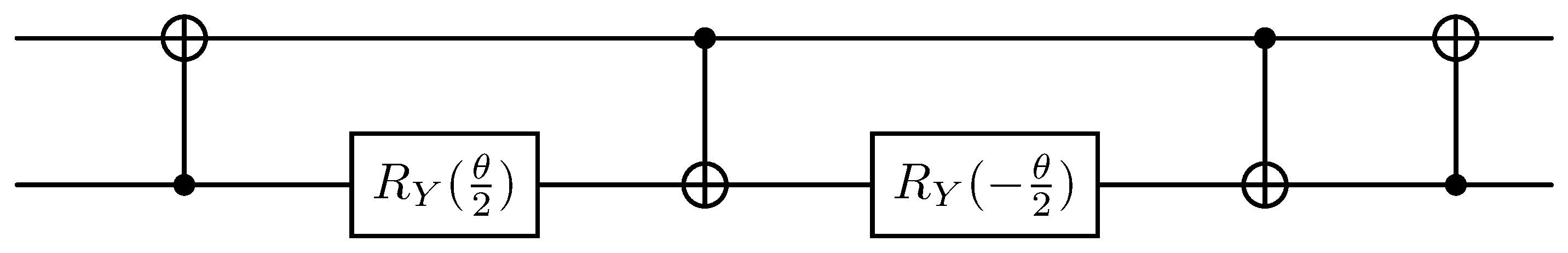
../../_images/givens.png — Fig. 25 Givens implementation using CNOTs and \(R_Y\) gates.¶

When \(\mathbf{K}\) contains imaginary or complex entries, a generalization of the QR-like is required [54]. This finds a sequence of rotations and phases that diagonalize the orbital rotation matrix which are the entries in the generalized Givens matrix, and the diagonal elements implemented as phases.

(110)¶\[\begin{split}\tilde{G}(\theta,\psi) = \begin{pmatrix} 1 & 0 & 0 & 0\\ 0 & \cos(-\theta) & -\sin(-\theta)\exp(-i\psi) & 0\\ 0 & \sin(-\theta)\exp(i\psi) & \cos(-\theta) & 0\\ 0 & 0 & 0 & 1 \end{pmatrix}\end{split}\]

Again, the inverse decomposition must be applied so \(\theta\) is negated. When \(\psi=0\), this recovers the same Givens matrix as before.

This matrix can be implemented with CNOT gates sandwiching CU3 and CU1 gates [56]. These gates are generic one qubit rotations, with the U3 rotating over all three axes, and U1 around the z-axis only. This differs from \(R_Z\) by a phase factor.

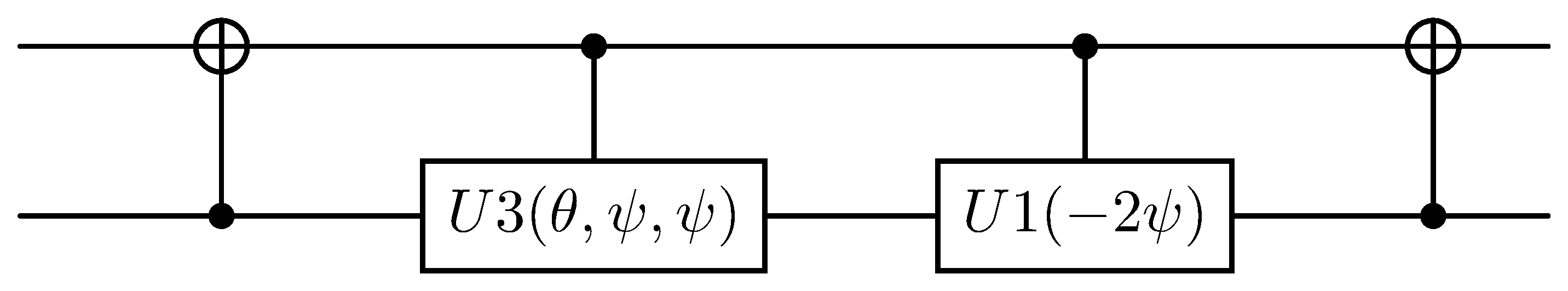
../../_images/generalized_givens.png — Fig. 26 Generalized Givens implementation using CNOTs and CU3 and CU1 gates.¶

This exact implementation has a slightly different design flow to other ansatzes, as the ansatz parameters are not trivially linked to ones that go into the circuit. This is due to the non-linear conversion of the fermionic orbital rotation parameters defined in Eq. (107) through the QR-like decompositions into the \(\theta,\psi\) parameters shown in Eq. (109) and Eq. (110), which is highlighted in the code snippet. The corresponding pytket circuit is also visualized. The phase gates rendered at the start of the figures below will typically be compiled together.

from inquanto.states import FermionState
from inquanto.spaces import FermionSpace
from inquanto.ansatzes import UnitaryClusterJastrowAnsatz, UnitaryClusterJastrowModel
from pytket.circuit.display import render_circuit_jupyter as draw

space, state = FermionSpace(4), FermionState([1,1,0,0])

for m in UnitaryClusterJastrowModel:
    ansatz = UnitaryClusterJastrowAnsatz(state, mode=m, k=1)
    print(f"{m=}\n{ansatz.generate_report()}\n{len(ansatz.free_symbols())=}")
    ansatz_params = ansatz.state_symbols.construct_random(sigma=0.1)
    circuit_params = ansatz.map_ansatz_parameters_to_circuit_parameters(ansatz_params)
    print(f"{ansatz_params=}\n{circuit_params=}\n\n")
    draw(ansatz.state_circuit)

m=<UnitaryClusterJastrowModel.REAL_K: 'real_k'>
{'n_parameters': 8, 'n_qubits': 4}
len(ansatz.free_symbols())=8
ansatz_params={Im-(J0)_{0}^{1}: 0.09417154046806644, Im-(J0)_{0}^{2}: -0.139657810470115, Im-(J0)_{0}^{3}: -0.0679714448078421, Im-(J0)_{1}^{2}: 0.037050356746065986, Im-(J0)_{1}^{3}: -0.1016348894188071, Im-(J0)_{2}^{3}: -0.007212002278507135, Re-(K0)_{0}^{2}: 0.01791964872748569, Re-(K0)_{1}^{3}: -0.08310992152709883}
circuit_params={(K0+phi)_{0}^{0}: np.float64(0.0), (K0+phi)_{1}^{1}: np.float64(1.0), (K0+phi)_{2}^{2}: np.float64(1.0), (K0+phi)_{3}^{3}: np.float64(0.0), (K0+theta)_{0}^{3}: 0.0, (K0+theta)_{0}^{2}: 0.5, (K0+theta)_{0}^{1}: np.complex128(-0.005704001346899478+0j), (K0+theta)_{1}^{3}: np.complex128(-0.026454709662034604+0j), (K0+theta)_{1}^{2}: 0.5, (K0+theta)_{2}^{3}: 0.0, (J0)_{0}^{1}: np.float64(-0.02997573232814247), (J0)_{0}^{2}: np.float64(0.044454461755419714), (J0)_{1}^{2}: np.float64(-0.011793494838909105), (J0)_{0}^{3}: np.float64(0.02163598286053203), (J0)_{1}^{3}: np.float64(0.03235139008320264), (J0)_{2}^{3}: np.float64(0.002295651624428845), (K0-phi)_{0}^{0}: np.float64(0.0), (K0-phi)_{1}^{1}: np.float64(1.0), (K0-phi)_{2}^{2}: np.float64(1.0), (K0-phi)_{3}^{3}: np.float64(0.0), (K0-theta)_{0}^{3}: 0.0, (K0-theta)_{0}^{2}: 0.5, (K0-theta)_{0}^{1}: np.complex128(0.005704001346899478+0j), (K0-theta)_{1}^{3}: np.complex128(0.026454709662034604+0j), (K0-theta)_{1}^{2}: 0.5, (K0-theta)_{2}^{3}: 0.0}

m=<UnitaryClusterJastrowModel.IMAGINARY_K: 'imaginary_k'>
{'n_parameters': 8, 'n_qubits': 4}
len(ansatz.free_symbols())=8
ansatz_params={Im-(J0)_{0}^{1}: 0.09417154046806644, Im-(J0)_{0}^{2}: -0.139657810470115, Im-(J0)_{0}^{3}: -0.0679714448078421, Im-(J0)_{1}^{2}: 0.037050356746065986, Im-(J0)_{1}^{3}: -0.1016348894188071, Im-(J0)_{2}^{3}: -0.007212002278507135, Im-(K0)_{0}^{2}: 0.01791964872748569, Im-(K0)_{1}^{3}: -0.08310992152709883}
circuit_params={(K0+phi)_{0}^{0}: np.float64(-6.258114157291452e-21), (K0+phi)_{1}^{1}: np.float64(1.0), (K0+phi)_{2}^{2}: np.float64(-1.0), (K0+phi)_{3}^{3}: np.float64(1.3431872768800994e-19), (K0+theta)_{0}^{3}: -0.0, (K0+psi)_{0}^{3}: -0.0, (K0+theta)_{0}^{2}: -1.0, (K0+psi)_{0}^{2}: -0.0, (K0+theta)_{0}^{1}: np.float64(0.01140800269379896), (K0+psi)_{0}^{1}: np.float64(0.5), (K0+theta)_{1}^{3}: np.float64(0.052909419324069215), (K0+psi)_{1}^{3}: np.float64(0.5), (K0+theta)_{1}^{2}: -1.0, (K0+psi)_{1}^{2}: -0.0, (K0+theta)_{2}^{3}: -0.0, (K0+psi)_{2}^{3}: -0.0, (J0)_{0}^{1}: np.float64(-0.02997573232814247), (J0)_{0}^{2}: np.float64(0.044454461755419714), (J0)_{1}^{2}: np.float64(-0.011793494838909105), (J0)_{0}^{3}: np.float64(0.02163598286053203), (J0)_{1}^{3}: np.float64(0.03235139008320264), (J0)_{2}^{3}: np.float64(0.002295651624428845), (K0-phi)_{0}^{0}: np.float64(6.258114157291452e-21), (K0-phi)_{1}^{1}: np.float64(-1.0), (K0-phi)_{2}^{2}: np.float64(1.0), (K0-phi)_{3}^{3}: np.float64(-1.3431872768800994e-19), (K0-theta)_{0}^{3}: -0.0, (K0-psi)_{0}^{3}: -0.0, (K0-theta)_{0}^{2}: -1.0, (K0-psi)_{0}^{2}: -0.0, (K0-theta)_{0}^{1}: np.float64(0.01140800269379896), (K0-psi)_{0}^{1}: np.float64(-0.5), (K0-theta)_{1}^{3}: np.float64(0.052909419324069215), (K0-psi)_{1}^{3}: np.float64(-0.5), (K0-theta)_{1}^{2}: -1.0, (K0-psi)_{1}^{2}: -0.0, (K0-theta)_{2}^{3}: -0.0, (K0-psi)_{2}^{3}: -0.0}

m=<UnitaryClusterJastrowModel.GENERAL_K: 'general_k'>
{'n_parameters': 10, 'n_qubits': 4}
len(ansatz.free_symbols())=10
ansatz_params={Im-(J0)_{0}^{1}: 0.09417154046806644, Im-(J0)_{0}^{2}: -0.139657810470115, Im-(J0)_{0}^{3}: -0.0679714448078421, Im-(J0)_{1}^{2}: 0.037050356746065986, Im-(J0)_{1}^{3}: -0.1016348894188071, Im-(J0)_{2}^{3}: -0.007212002278507135, Im-(K0)_{0}^{2}: 0.01791964872748569, Im-(K0)_{1}^{3}: -0.08310992152709883, Re-(K0)_{0}^{2}: -0.13090373644593586, Re-(K0)_{1}^{3}: 0.019388774124910413}
circuit_params={(K0+phi)_{0}^{0}: np.float64(-1.3804490804963183e-19), (K0+phi)_{1}^{1}: np.float64(1.0), (K0+phi)_{2}^{2}: np.float64(-1.0), (K0+phi)_{3}^{3}: np.float64(-6.90224540248159e-20), (K0+theta)_{0}^{3}: -0.0, (K0+psi)_{0}^{3}: -0.0, (K0+theta)_{0}^{2}: -1.0, (K0+psi)_{0}^{2}: -0.0, (K0+theta)_{0}^{1}: np.float64(0.08411311374583698), (K0+psi)_{0}^{1}: np.float64(0.9566951484095471), (K0+theta)_{1}^{3}: np.float64(0.05433013104682823), (K0+psi)_{1}^{3}: np.float64(0.5729539291073631), (K0+theta)_{1}^{2}: -1.0, (K0+psi)_{1}^{2}: -0.0, (K0+theta)_{2}^{3}: -0.0, (K0+psi)_{2}^{3}: -0.0, (J0)_{0}^{1}: np.float64(-0.02997573232814247), (J0)_{0}^{2}: np.float64(0.044454461755419714), (J0)_{1}^{2}: np.float64(-0.011793494838909105), (J0)_{0}^{3}: np.float64(0.02163598286053203), (J0)_{1}^{3}: np.float64(0.03235139008320264), (J0)_{2}^{3}: np.float64(0.002295651624428845), (K0-phi)_{0}^{0}: np.float64(0.0), (K0-phi)_{1}^{1}: np.float64(-1.0), (K0-phi)_{2}^{2}: np.float64(1.0), (K0-phi)_{3}^{3}: np.float64(-2.760898160992636e-19), (K0-theta)_{0}^{3}: -0.0, (K0-psi)_{0}^{3}: -0.0, (K0-theta)_{0}^{2}: -1.0, (K0-psi)_{0}^{2}: -0.0, (K0-theta)_{0}^{1}: np.float64(0.08411311374583698), (K0-psi)_{0}^{1}: np.float64(-0.04330485159045297), (K0-theta)_{1}^{3}: np.float64(0.05433013104682823), (K0-psi)_{1}^{3}: np.float64(-0.4270460708926369), (K0-theta)_{1}^{2}: -1.0, (K0-psi)_{1}^{2}: -0.0, (K0-theta)_{2}^{3}: -0.0, (K0-psi)_{2}^{3}: -0.0}

The ansatz parameters are given chemically meaningful symbols as they represent the type of excitation they are carrying out. In both UnitaryClusterJastrowAnsatz (which does not suffer from Trotter error) and FermionSpaceAnsatzUnitaryClusterJastrow, the symbols are constructed as \(\text{NumType}-\mathbf{M}\text{k}_\text{LowerSpinorb}^{\text{HigherSpinorb}}\) where \(\text{NumType}\) is either \(\text{Re}\) for a real parameter or \(\text{Im}\) for an imaginary, \(\mathbf{M}\) is either \(\mathbf{K}\) or \(\mathbf{J}\) for the operator it refers to an \(\text{k}\) is the repeat index.

The reason to go through this decomposition procedure is to avoid the Trotter error inherently present when using the fermionic version of this ansatz. This ansatz circumvents this by directly manipulating the orbital rotation matrix itself and converting those parameters into gates on the circuit.

A major caveat with both versions of this ansatz is that using them for VQE is extremely sensitive to the minimizer used, as well as the initial parameters. The ucJ ansatz does have a tendency to get stuck in the Hartree–Fock reference state, and with the fermionic implementation it is recommended to have random initial parameters away from zeros. Conversely, for the exact implementation it is recommended to have initial parameters closer to zero, especially for the GENERAL_K version for stability.