Unitary Product State
A first order Trotter expansion has the following effect:
where \(\hat{\kappa}\) is a generalized fermionic excitation operator,
and \(\theta_I\) is a variational parameter (N.B. ordering of indices in \(\hat{\kappa}\) ). Traditional UCC expresses its ansatz as the left hand side of this approximation, while it is canonically implemented as the right hand side, which has been referred to as disentangled UCC (dUCC). [50]
However, we can equally define an ansatz to be the right hand side, denoted as a Unitary Product State (UPS). [51, 52]. What would usually be called a Trotter error, can be considered to be an operator ordering error.
The following UPS ansatze are available in InQuanto:
Symmetrized [51]
FermionSpaceAnsatzsUPSTiled [52]
FermionSpaceAnsatztUPS
They are further elaborated in the corresponding subsections.
Symmetry Preserving UPS (sUPS)
By restricting the operators
where \(p,q\) are spatial orbital indices which can include occupied-to-occupied and virtual-to-virtual transitions, and \(\alpha, \beta\) index spins. By only using spin adapted singles and paired doubles, the spin symmetry of the initial state is preserved.
In the DISCO-VQE algorithm [51], the optimal sequence of operators
is found through a discrete optimization technique. This sequence (or any other) can be provided
to FermionSpaceAnsatzsUPS, otherwise one copy of the spin adapted singles
and paired doubles is used, which makes the ansatz equivalent to the
FermionSpaceAnsatzkUpCCGSDSinglet ansatz with \(k=1\).
The following code snippet can construct the optimal ordered ansatz for linear H \(_4\).
from inquanto.states import FermionState
from inquanto.spaces import FermionSpace
from inquanto.ansatzes import FermionSpaceAnsatzsUPS

space = FermionSpace(8)
state = FermionState([1, 1, 1, 1, 0, 0, 0, 0])

excitations = [
    ("s", 1, 2),
    ("d", 1, 2),
    ("d", 0, 3),
    ("d", 2, 3),
    ("s", 0, 3),
    ("d", 0, 3),
    ("s", 0, 2),
    ("d", 0, 3),
    ("s", 1, 3),
    ("d", 1, 3),
    ("d", 0, 3),
    ("s", 1, 3),
    ("d", 0, 1),
]

sups_ansatz_optimal = FermionSpaceAnsatzsUPS(space, state, excitations)
sups_ansatz = FermionSpaceAnsatzsUPS(space, state)

print("\nNumber of parameters: {} (sUPS), {} (optimal sUPS)".format(
    sups_ansatz.generate_report()['n_parameters'],
    sups_ansatz_optimal.generate_report()['n_parameters'])
)
Number of parameters: 12 (sUPS), 13 (optimal sUPS)
The excitations are indexed by 3 parameters: the type of excitation (a single or double)
denoted by s and d respectively, the index of the spatial orbital to annihilate
electrons from, and the index of the spatial orbital to create electrons in. These are 0-indexed.
Setting excitations=None which is its default value, will revert to
FermionSpaceAnsatzkUpCCGSDSinglet with \(k=1\).
Tiled UPS (tUPS)
While the FermionSpaceAnsatzsUPS ansatz requires a priori knowledge
of the precise operators to use within the ansatz, FermionSpaceAnsatztUPS
removes this necessity by building an ansatz using a tiled structure shown in Fig. 23.
In the examples below we examine CH \(_2\) with an active space of 6 electrons in 6 spatial orbitals.
This is due to the importance of the singlet and triplet ground states.
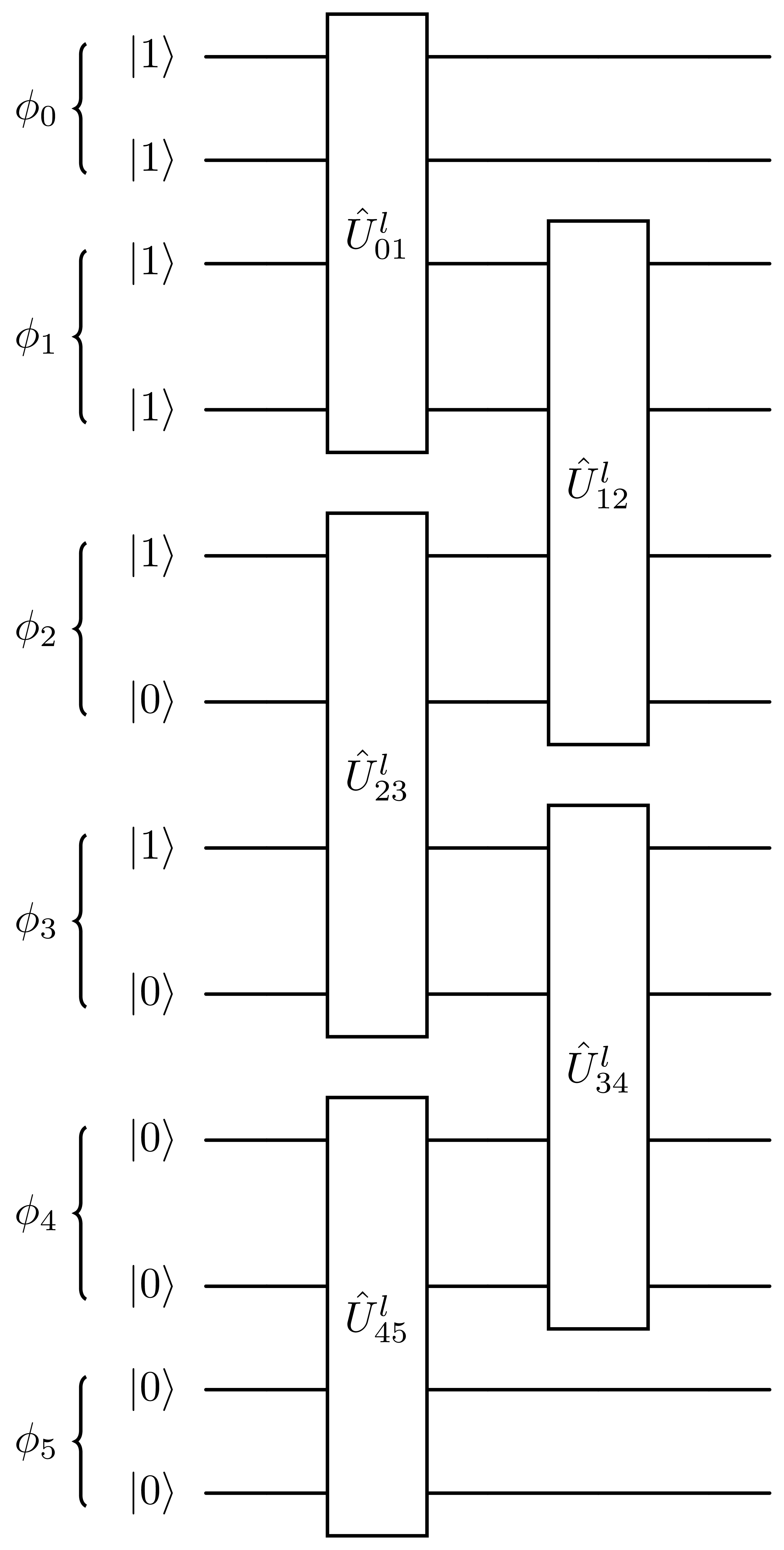
Fig. 23 1 layer of a tUPS circuit.
The operator within each tile is defined by
which combines a single, double and single excitation between spatial orbitals \(p,q\) in each
layer \(l\). This layer can be repeated multiple times, analogous to the
FermionSpaceAnsatzkUpCCGSD type ansatze.
To improve the ground state energy, orbital optimization can be performed. While this can be done classically by rotating the one-electron and two-electron integrals, at the circuit level this can be achieved by appending an analogous type of circuit in Fig. 23 by replacing the operators with
The number of layers in this orbital optimization circuit is fixed at \(\lfloor\frac{N}{2}\rfloor\) (the rounded down integer) where \(N\) is the number of spatial orbitals in the system.
To maximize the amount of entanglement in the first layer, the operators \(\hat{U}\) should link occupied and virtual orbitals. This is equivalent to perfect pairing theory, and can be achieved by “moving” the orbitals to be linked together to be nearest neighbors. An example of this transformation is shown in Fig. 24.
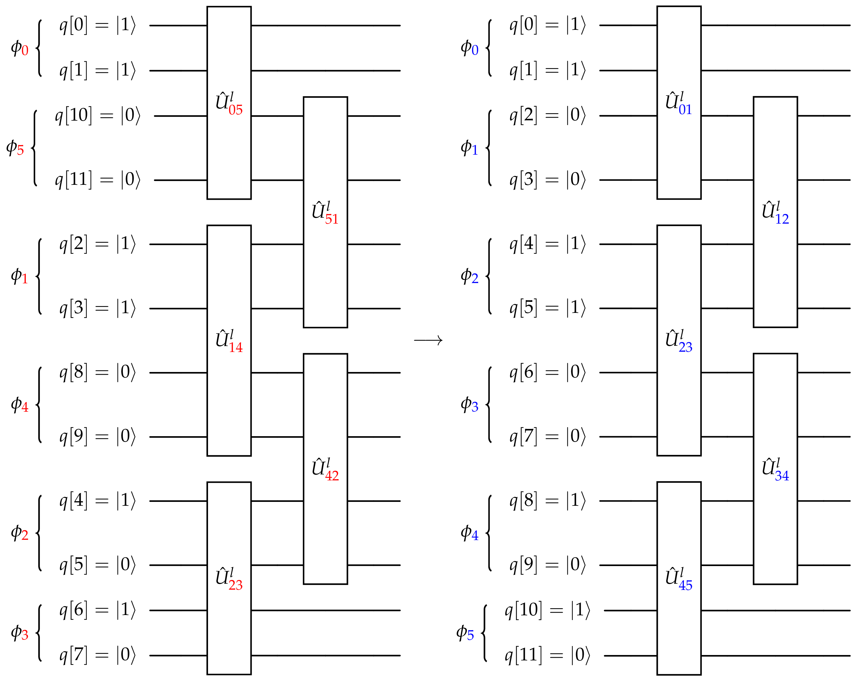
Fig. 24 Demonstration of the perfect-pairing process and the tUPS circuit with 1 layer.
The perfect pairing procedure matches the lowest energy spatial orbital with the highest, and folds inwards. The spatial
indices in red (left) are permuted to the ones in blue (as spin orbitals) using the
permuted_operator() method with a dictionary mapping the
spin-orbital index to the qubit index. When using this, the Hamiltonian must also be permuted at the
fermionic level also using this mapping, and the fermion state also re-ordered.
The reason to permute at the fermion level becomes apparent when observing the qubit indices on the left ansatz in Fig. 24, where the single excitations in the \(\hat{U}^l_{\color{red}05}\) box link qubit indices 0, 1, 10, 11 which introduces extra Z strings and subsequently extra 2-qubit gate counts, which is alleviated by this permutation at the fermionic level.
Perfect pairing is implemented using the enum PerfectPairing and takes
2 values: NONE and ORBITAL_ENERGY.
Because this ansatz only uses fermionic operators that maintain spin symmetry, different spin states can be targeted, such as the singlet and triplet of CH \(_2\). This is highlighted in the following code snippet.
from inquanto.states import FermionState
from inquanto.spaces import FermionSpace
from inquanto.ansatzes import FermionSpaceAnsatztUPS, PerfectPairing

space = FermionSpace(12)
singlet_state = FermionState([1, 1, 1, 1, 1, 1, 0, 0, 0, 0, 0, 0])
triplet_state = FermionState([1, 1, 1, 1, 1, 0, 1, 0, 0, 0, 0, 0])

for layers in range(1,4):
    for oo in [False, True]:
        for pp in PerfectPairing:
            if not oo and pp!=PerfectPairing.NONE: # perfect pairing usually only on top of oo
                continue

            singlet_ansatz_tups = FermionSpaceAnsatztUPS(space, singlet_state, layers, oo, pp)
            triplet_ansatz_tups = FermionSpaceAnsatztUPS(space, triplet_state, layers, oo, pp)

            singlet_resources = singlet_ansatz_tups.generate_report()
            triplet_resources = triplet_ansatz_tups.generate_report()

            print(
                f"Layers:{layers} \t Orbital Optimization:{oo} \t Perfect Pairing:{pp}",
                f"{singlet_resources=}\n{triplet_resources=}"
            )
Layers:1 	 Orbital Optimization:False 	 Perfect Pairing:PerfectPairing.NONE singlet_resources={'n_parameters': 15, 'n_qubits': 12}
triplet_resources={'n_parameters': 15, 'n_qubits': 12}
Layers:1 	 Orbital Optimization:True 	 Perfect Pairing:PerfectPairing.NONE singlet_resources={'n_parameters': 30, 'n_qubits': 12}
triplet_resources={'n_parameters': 30, 'n_qubits': 12}
Layers:1 	 Orbital Optimization:True 	 Perfect Pairing:PerfectPairing.ORBITAL_ENERGY singlet_resources={'n_parameters': 30, 'n_qubits': 12}
triplet_resources={'n_parameters': 30, 'n_qubits': 12}
Layers:2 	 Orbital Optimization:False 	 Perfect Pairing:PerfectPairing.NONE singlet_resources={'n_parameters': 30, 'n_qubits': 12}
triplet_resources={'n_parameters': 30, 'n_qubits': 12}
Layers:2 	 Orbital Optimization:True 	 Perfect Pairing:PerfectPairing.NONE singlet_resources={'n_parameters': 45, 'n_qubits': 12}
triplet_resources={'n_parameters': 45, 'n_qubits': 12}
Layers:2 	 Orbital Optimization:True 	 Perfect Pairing:PerfectPairing.ORBITAL_ENERGY singlet_resources={'n_parameters': 45, 'n_qubits': 12}
triplet_resources={'n_parameters': 45, 'n_qubits': 12}
Layers:3 	 Orbital Optimization:False 	 Perfect Pairing:PerfectPairing.NONE singlet_resources={'n_parameters': 45, 'n_qubits': 12}
triplet_resources={'n_parameters': 45, 'n_qubits': 12}
Layers:3 	 Orbital Optimization:True 	 Perfect Pairing:PerfectPairing.NONE singlet_resources={'n_parameters': 60, 'n_qubits': 12}
triplet_resources={'n_parameters': 60, 'n_qubits': 12}
Layers:3 	 Orbital Optimization:True 	 Perfect Pairing:PerfectPairing.ORBITAL_ENERGY
singlet_resources={'n_parameters': 60, 'n_qubits': 12}
triplet_resources={'n_parameters': 60, 'n_qubits': 12}