System Operation

The operation of quantum computers requires multiple compilations of quantum programs to lower levels, regular maintece of the machine, calibrations, and performance validations. Details on system operation are provided below.

Full-stack Operation

The table below details job lifecycle and system operation from the end user level to execution on the commercial quantum computer. The tasking and operations layer manages and allocates access to the system, whilst the machine control and real-time execution layer manages and maintain system performance. Specifically for on-premises deployment, tasking and operations, machine control and real-time execution layers are bundled together in the system.

Layer	Details
Application Layer	End User creates program and submits job. Generate quantum program with Guppy Language Send to emulator or hardware (Nexus) Receive and process results (Nexus)
Access Layer	Provide stable access API to customers: Enable fine-grained job management and visibility Support usage metering and billing Handle authentication and authorization
Tasking and Operations Layer	Compile user programs Optimize quantum circuits (TKET) Compile to machine code (pulse control) Distribute workload to different QPU's Provide operator interface
Machine Control Layer	Compose real-time sequences Schedule calibrations and user jobs Monitor and control lab instruments Maintain and validate QPU state
Real Time Execution Layer	Execute real-time sequences of commands Actuate control signals Retrieve measurement results

Job Chunking and Performance Validation

Jobs submitted with large shot counts are automatically divided into appropriately sized chunks of smaller shot counts in a method called chunking. Chunking ensures that system state checks and dynamic calibrations happen at the appropriate frequency. The number of shots in a chunk is dynamically chosen by the machine control layer and is determined by the estimated shot time calculated by the compiler. A series of system checks are performed before and after each chunk. If an error is detected, any suspect results are rejected, and the failed chunk shots are rerun at no additional cost. The job start time indicates the start of the first chunk and the job stop time indicates the end of the last chunk. This means that the total job duration includes system checks, calibrations, and, for multi-chunk jobs, possibly interleaved chunks from other jobs in the queue.

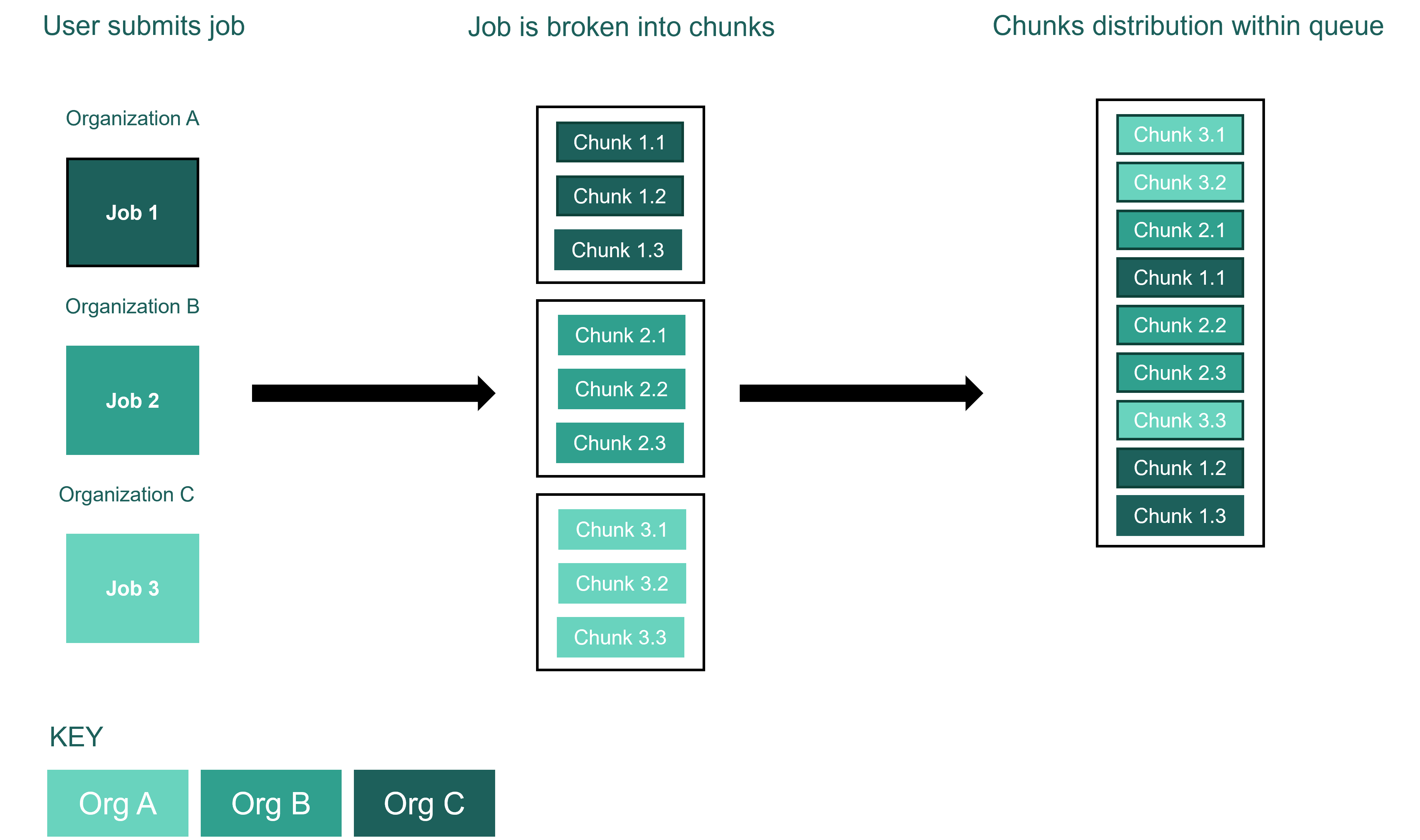
Chunking of a job, submitted to the Quantinuum queue, by a user in Organisation A.

A variety of system actions are performed during chunking. This is to ensure optimal system performance across the chunks of a job. These actions are reported in the table below. There are four types of actions: checks, calibrations, validations and interventions.

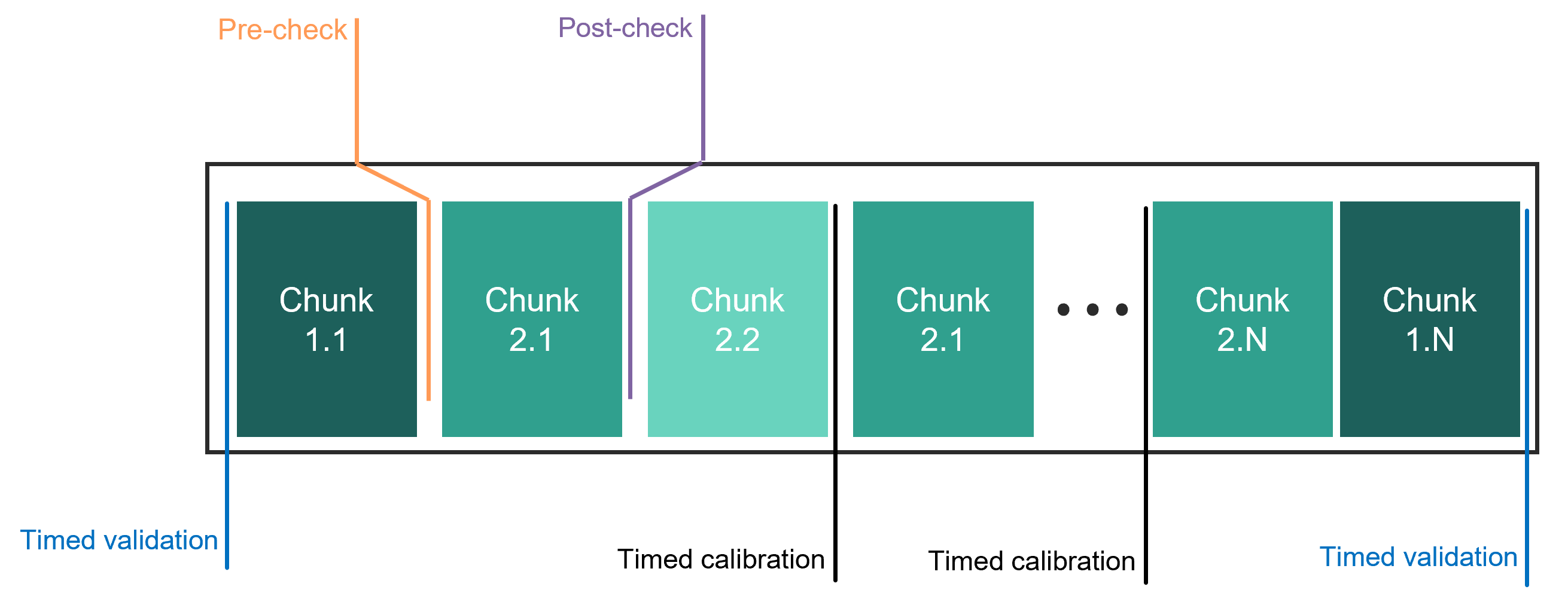
System actions to maintain performance. System checks, validations and calibrations are performed across the job chunks in the queue.

Action	Description
Pre-checks	before a chunk, e.g., check ion number, crystal order, B-field baselines; intervene (automatic or operator) as needed
Post-checks	after a chunk, e.g., check ion number, crystal order, B-field baselines; if incorrect, throw out data, intervene, and rerun chunk; ensure B-field difference pre- and post-chunk execution is negligible
Timed calibrations	interleave with chunks based on dynamically characterized calibration schedule
Timed validations	interleave with chunks based on dynamically characterized validation schedule
Automatic interventions	performed dynamically or as response to failed checks and calibration or validation issues, e.g., load more ions
Operator (human) interventions	performed in response to failed checks and calibration or validation issues when the machine control layer is unable to automatically self-correct, e.g., a non-computer-controlled component requires attention

The schematic above shows when the system checks, validations and calibrations are performed across the job chunks in the queue. The system automatically schedules and executes calibration routines. There are two types of automated calibrations: those that are executed on a predetermined time interval and those that are triggered when a drift tolerance is exceeded. Because the latter does not follow a predetermined schedule, the circuit throughput and execution time will vary due to these calibrations. The schematic below shows triggered intervention when a system check fails. The triggered intervention performs a system-correcting action, so that operation can continue with satisfactory performance.

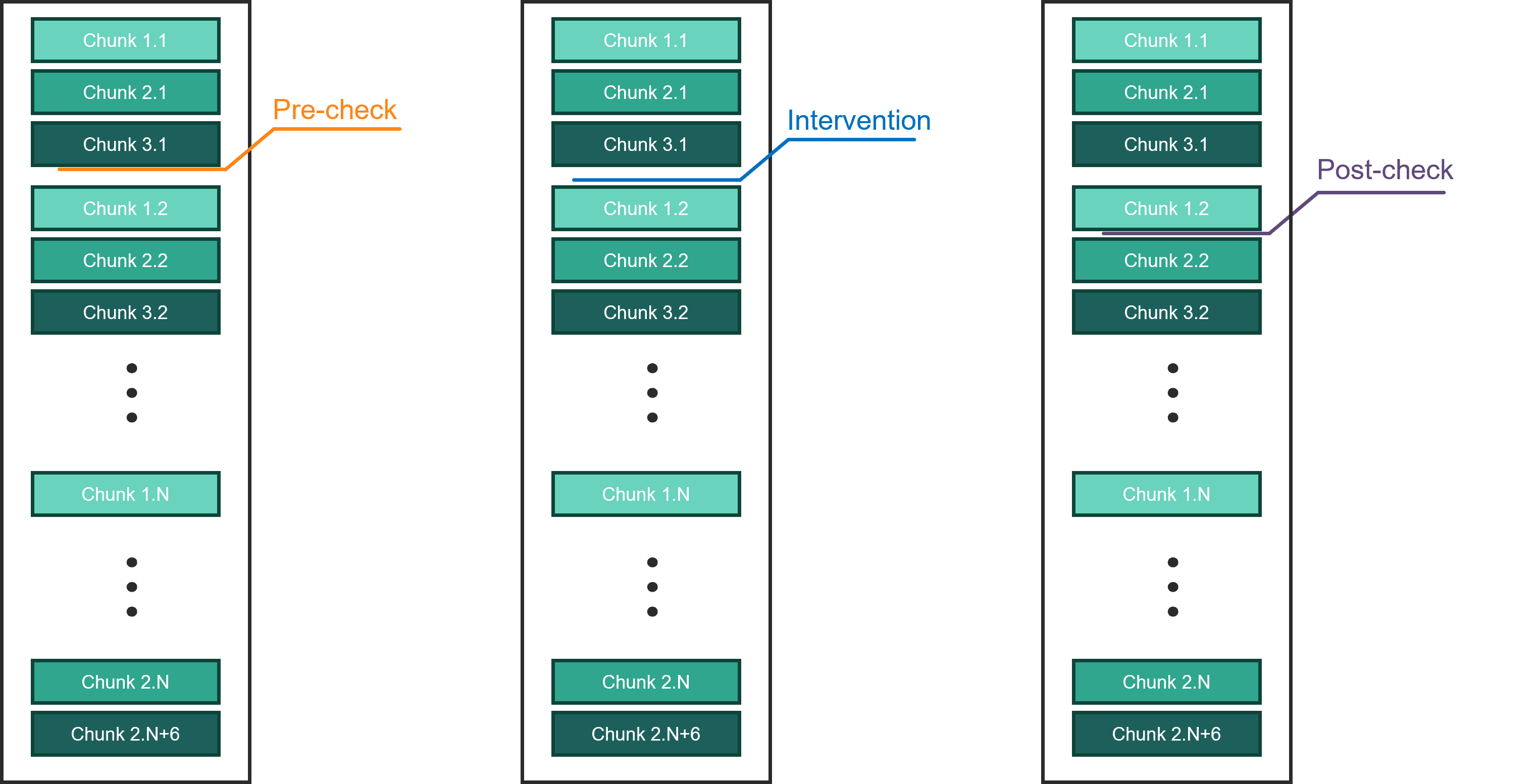
System actions to maintain performance. Triggered intervention to perform system-correcting action when pre-checks fail.

Depth-1 Circuit Time

We define the depth-1 circuit time as the time it takes to arbitrarily permute all qubits and perform 1-qubit and 2-qubit gates on all \(\left[(N/2)\right]\) pairs for a maximally dense circuit, as shown in Figure 1, where \(P\) represents the random permutation of all qubits. For maximally dense circuits the gating rate and the idle time for any qubit can both be directly calculated from the depth-1 circuit time. However, for less dense circuits with different numbers of qubits, the gate rate and idle time per qubit will differ from the depth-1 circuit time.

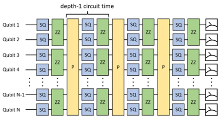
Depth-1 circuit time for a maximally dense circuit.

References