System Operation
The operation of quantum computers requires multiple compilations of quantum programs to lower levels, regular maintenance of the machine, calibrations, and performance validations. Details on system operation are provided below.
Full-stack Operation
The table below details job lifecyle and system operation from the end user level to execution on the commercial quantum computer. The tasking and operations layer manages and allocates access to the system, whilst the machine control and real-time execution layer manages and maintain system performance. Specifically for on-premises deployment, tasking and operations, machine control and real-time execution layers are bundled together in the system.
| Layer | Details |
|---|---|
Application Layer |
End User creates program and submits job.
|
Access Layer
|
Provide stable access API to customers:
|
Tasking and Operations Layer
|
|
Machine Control Layer
|
|
Real Time Execution Layer
|
|
Job Chunking and Performance Validation
Jobs submitted with large shot counts are automatically divided into appropriately sized chunks of smaller shot counts in a method called chunking. Chunking ensures that system state checks and dynamic calibrations happen at the appropriate frequency. The number of shots in a chunk is dynamically chosen by the machine control layer and is determined by the estimated shot time calculated by the compiler. A series of system checks are performed before and after each chunk. If an error is detected, any suspect results are rejected, and the failed chunk shots are rerun at no additional cost. The job start time indicates the start of the first chunk and the job stop time indicates the end of the last chunk. This means that the total job duration includes system checks, calibrations, and, for multi-chunk jobs, possibly interleaved chunks from other jobs in the queue.
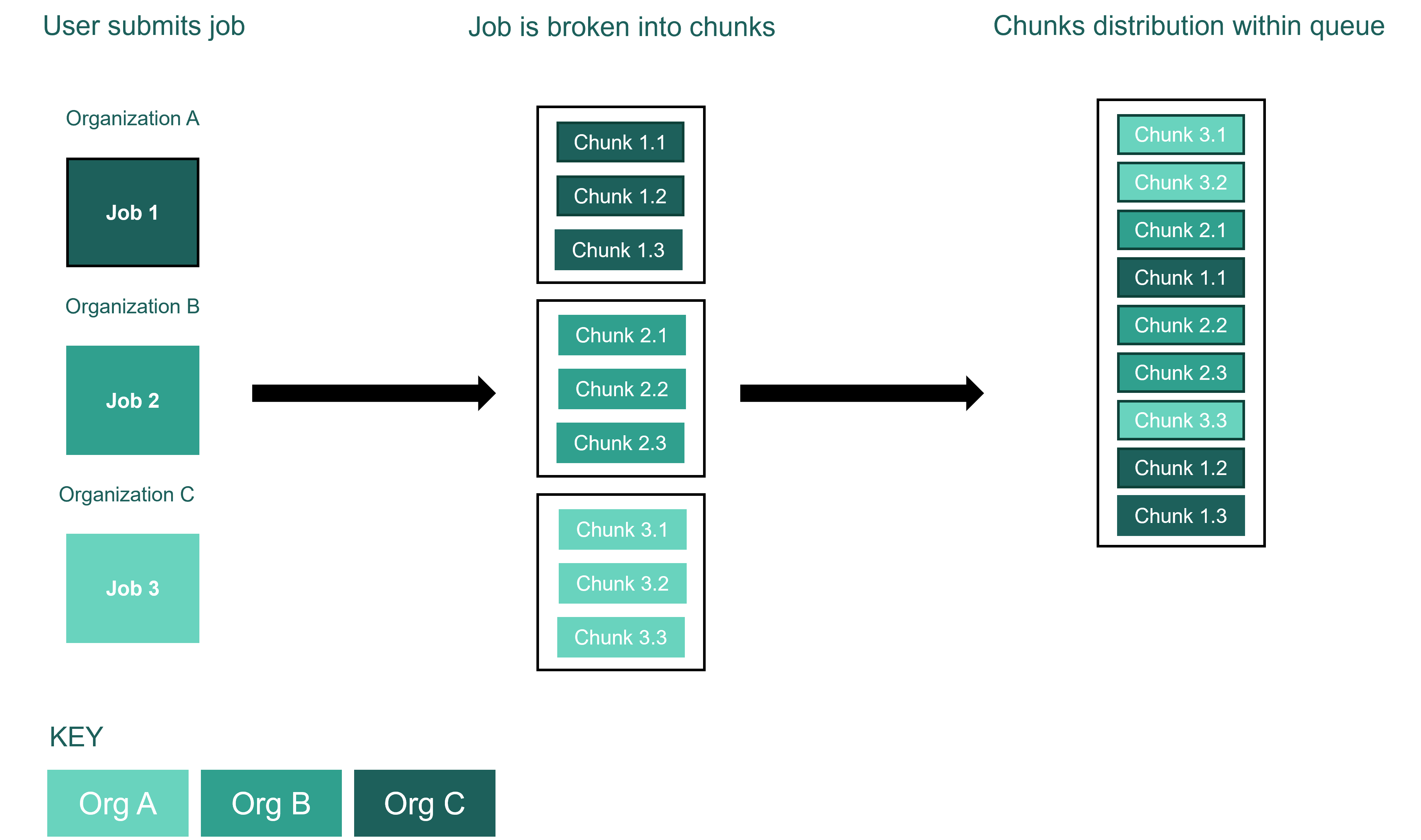
Chunking of a job, submitted to the Quantinuum queue, by a user in Organisation A.
A variety of system actions are performed during chunking. This is to ensure optimal system performance across the chunks of a job. These actions are reported in the table below. There are four types of actions: checks, calibrations, validations and interventions.
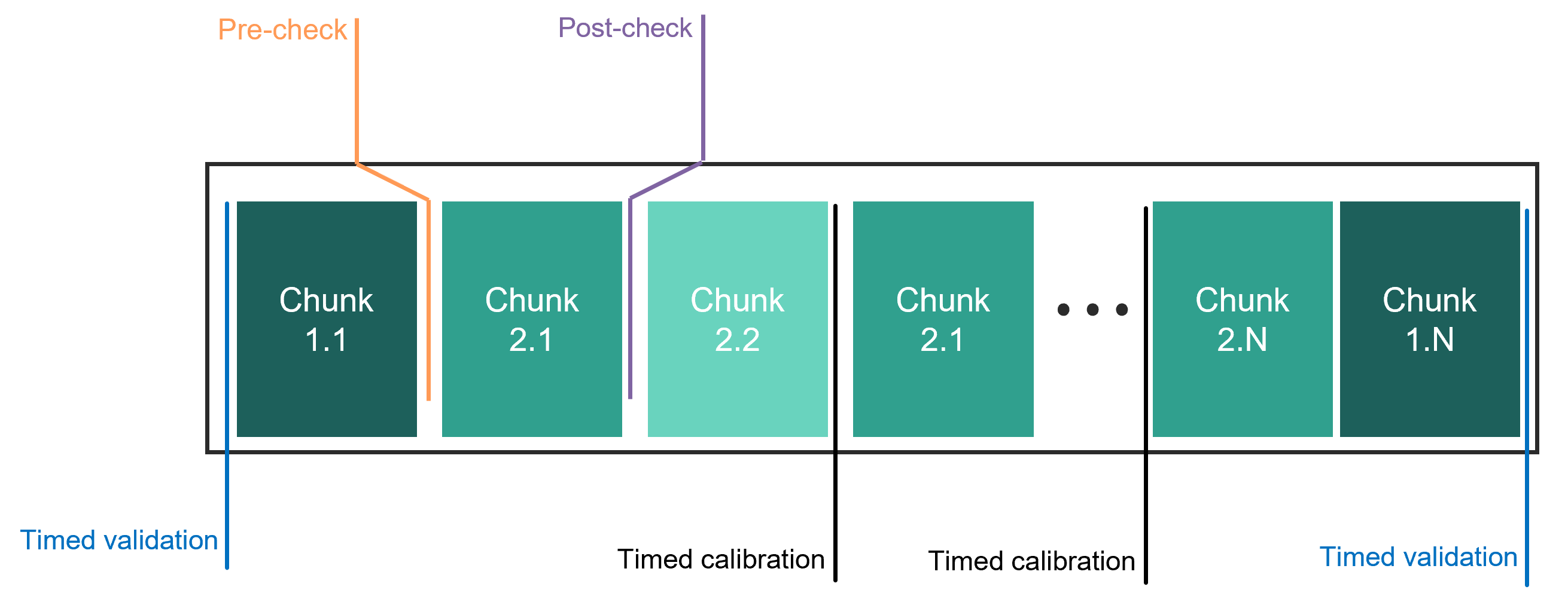
System actions to maintain performance. System checks, validations and calibrations are performed across the job chunks in the queue.
Action |
Description |
Pre-checks |
before a chunk, e.g., check ion number, crystal order, B-field baselines; intervene (automatic or operator) as needed |
Post-checks |
after a chunk, e.g., check ion number, crystal order, B-field baselines; if incorrect, throw out data, intervene, and rerun chunk; ensure B-field difference pre- and post-chunk execution is negligble |
Timed calibrations |
interleave with chunks based on dynamically characterized calibration schedule |
Timed validations |
interleave with chunks based on dynamically characterized validation schedule |
Automatic interventions |
performed dynamically or as response to failed checks and calibration or validation issues, e.g., load more ions |
Operator (human) interventions |
performed in response to failed checks and calibration or validation issues when the machine control layer is unable to automatically self-correct, e.g., a non-computer-controlled component requires attention |
The schematic above shows when the system checks, validations and calibrations are performed across the job chunks in the queue. The system automatically schedules and executes calibration routines. There are two types of automated calibrations: those that are executed on a predetermined time interval and those that are triggered when a drift tolerance is exceeded. Because the latter does not follow a predetermined schedule, the circuit throughput and execution time will vary due to these calibrations. The schematic below shows triggered intervention when a system check fails. The triggered intervention performs a system-correcting action, so that operation can continue with satisfactory performance.
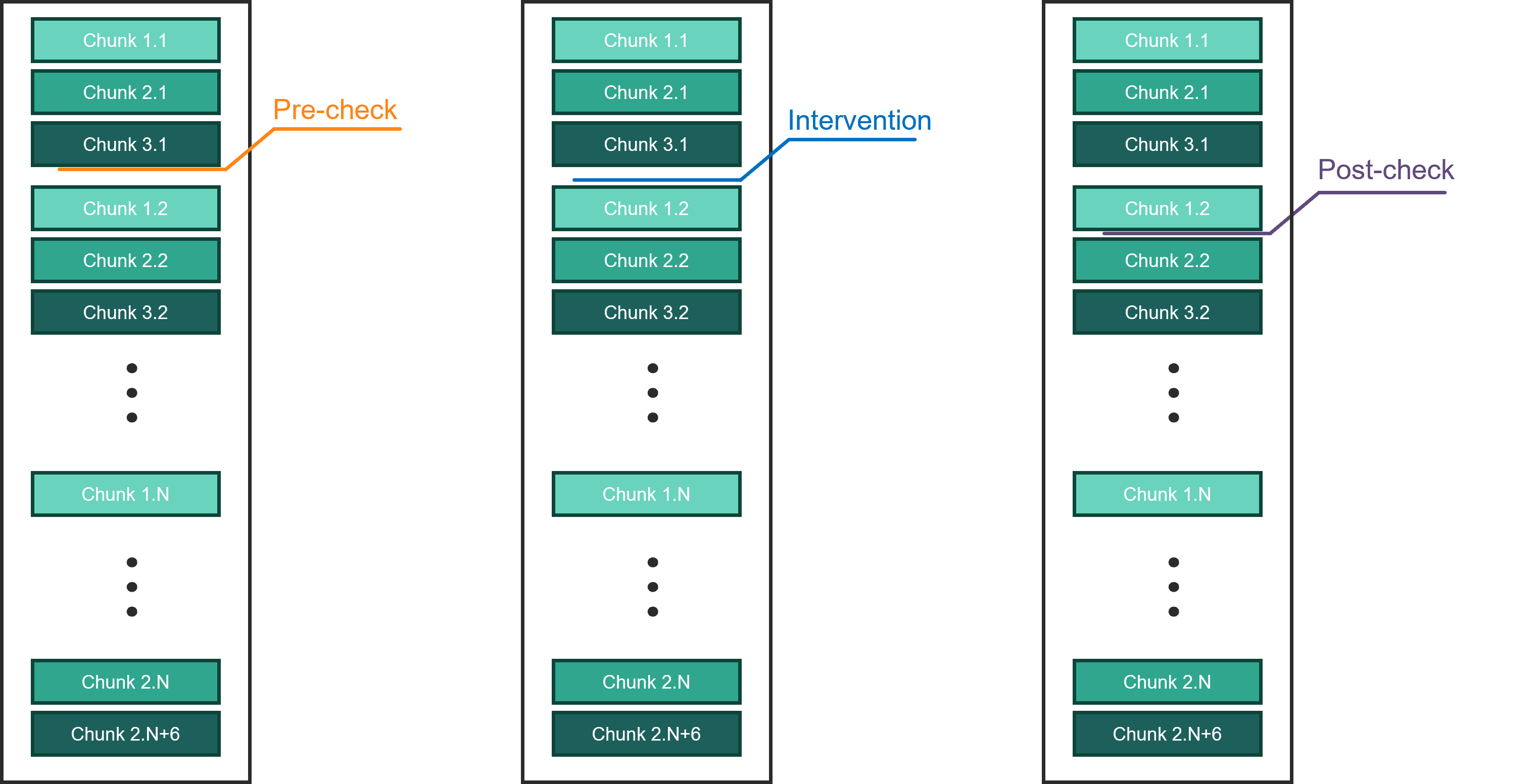
System actions to maintain performance. Triggered intervention to perform system-correcting action when pre-checks fail.
Native Gate Set
Quantinuum Hardware utilizes the following native gate set. The TKET definitions are in units of \(\pi\), but the formulas in the middle column are defined in radians.
Gate |
Expression |
TKET |
Native 1-qubit gates |
||
\(U_{1q} (\theta, \phi)\) |
\(e^{ \frac{-i \theta}{2} \left(\cos(\phi) \hat{X} + \sin(\phi) \hat{Y}\right) }\) |
|
\(R_{z}(\lambda)\) |
\(e^{-i \frac{\lambda}{2} \hat{Z}}\) |
|
Fully entangling 2-qubit gates |
||
\(ZZ()\) |
\(e^{-i \frac{\pi}{4} \hat{Z} \bigotimes \hat{Z}}\) |
|
Parameterized angle 2-qubit gates |
||
\(RZZ(\theta)\) |
\(e^{-i \frac{\theta}{2} \hat{Z} \bigotimes \hat{Z} }\) |
|
General SU(4) entangler |
||
\(Rxxyyzz (\alpha, \beta, \gamma)\) |
\(e^{\frac{-i}{2} (\alpha \hat{X} \bigotimes \hat{X} + \beta \hat{Y} \bigotimes \hat{Y} + \gamma \hat{Z} \bigotimes \hat{Z})}\) |
|
\(\hat{X}\), \(\hat{Y}\) and \(\hat{Z}\) are the standard Pauli operators, and the two-qubit matrix is written in the \(|0,0 \rangle\), \(|0,1 \rangle\), \(|1,0 \rangle\), \(|1,1 \rangle\) basis.
The parameterized rotation around the \(z\)-axis, \(R_z\) (\(\lambda\)), is performed virtually within the software. All other physical gates are constructed from this set.
By default, quantum circuits submitted to the hardware are rebased to the fully entangling \(ZZ\) gate and the parameterized \(RZZ\) gate. Circuits are rebased to the \(Rxxyyzz(\alpha, \beta, \gamma)\) only if users specify this option at job submission. The minimum gate angles for the \(RZZ\) gate angle is \(1 \times 10^{-4}\) and the minimum \(U_{1q}\) gate angle is \(3 \times 10^{-4}\). Gates angles smaller are automatically rounded to zero.
Note
Please note that our native \(U_1q(\theta, \phi)\) gate is NOT IBM’s standard \(U(\theta , \phi, \lambda)\)[1].
\(U_{1q} (\theta, \phi) = U \left( \theta, \phi - \frac{\pi}{2}, \frac{\pi}{2} - \phi \right)\).
Rebasing Quantum Circuits
Quantum circuits are rebased to the Quantinuum native gate set as described below.
Gate |
Rebase |
Pauli gate: bit-flip |
\(\sigma_x = U_{1q} (\pi,0)\) |
Pauli gate: bit and phase flip |
\(\sigma_y = U_{1q} (\pi,\pi/2)\) |
Pauli gate: phase flip |
\(\sigma_z = R_z(\pi)\) |
Clifford gate: Hadamard |
\(H = U_{1q} (\pi/2,-\pi/2)\) |
\(R_z(\pi)\) |
|
Clifford gate: CNOT |
\(CX^{(c,t)} = U_{1q}^{(t)}(-\pi/2,\pi/2)\) |
\(ZZ\) |
|
\(R_{z}^{(c)}(-\pi/2)\) |
|
\(U_{1q}^{(t)}(\pi/2,\pi)\) |
|
\(R_{z}^{(t)}(-\pi/2)\) |
|
Pauli interaction: Z basis |
\(R_{zz}(\pi/4) = Rzz(\pi/4)\) |
Pauli interaction: X basis |
\(R_{xx}(\pi/4) = U_{1q}^{(c)}(\pi/2,\pi/2)\) |
\(U_{1q}^{(t)}(\pi/2,\pi/2)\) |
|
\(R_{zz}(\pi/4)\) |
|
\(U_{1q}^{(c)}(\pi/2,-\pi/2)\) |
|
\(U_{1q}^{(t)}(\pi/2,-\pi/2)\) |
Mid-circuit Measurement and Conditional Operations
Due to the internal level structure of trapped-ion qubits, a mid-circuit measurement may leave the qubit in a non-computational state. All mid-circuit measurements should be followed by initialization if the qubit is to be used again in that circuit. The qubit may be prepared in the measured state by calling for a measurement followed by initialization and a measurement dependent spin-flip.
When a subset of qubits is measured in the middle of the circuit, the classical information from these measurements can be used to condition future elements of the circuit. Although the laser pulses that implement both 1- and 2-qubit gates are conditional, the transport operations used to rearrange the physical location of the qubits are not. The qubits will be reconfigured to allow for all gates in all branches irrespective of the mid-circuit measurement outcome. In the context of memory error and run time, the effective depth of a circuit with measurement conditioned branching includes all branches.
A discussion on mid-circuit measurement and reset consumption with pytket is available here.
Depth-1 Circuit Time
We define the depth-1 circuit time as the time it takes to arbitrarily permute all qubits and perform 1-qubit and 2-qubit gates on all \(\left[(N/2)\right]\) pairs for a maximally dense circuit, as shown in Figure 1, where \(P\) represents the random permutation of all qubits. System Model H1 requires 2 gating rounds to perform 10 pairwise 2-qubit gates across all qubits in a depth-1 circuit. Similarly, System Model H2 requires 7 gating rounds to apply 28 pairwise 2-qubit gate across all qubits in a depth-1 circuit. For maximally dense circuits the gating rate and the idle time for any qubit can both be directly calculated from the depth-1 circuit time. However, for less dense circuits with different numbers of qubits, the gate rate and idle time per qubit will differ from the depth-1 circuit time.
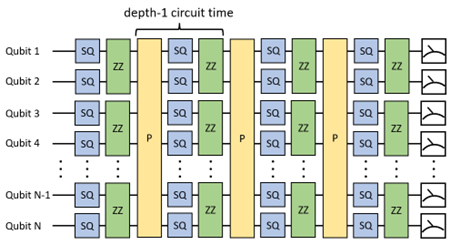
Depth-1 circuit time for a maximally dense circuit.
Hardware Credit Limitations
Each shot submitted to hardware has a 50 HQC hard limit. Each job submitted to hardware is limited to 10,000 shots (500,000 HQC hard limit). These cost restrictions ensure the chunk duration for each job does not exceed the maximum allowable interval between system checks, calibrations, and validations while ensuring system performance. Users are encouraged to contact Quantinuum to increase their HQC limits per shot.
Parameterized Angle ZZ Gates
Although a parameterized angle 2-qubit entangling gate can be constructed using two fixed-angle 2-qubit entangling gates, a direct implementation will lower the error rate in the circuit. Not only is the number of entangling gates reduced, but the error of an \(RZZ(\theta)\) gate also scales with the angle \(\theta\) [2]. The error on \(RZZ(\frac{\pi}{2})\) is equal to the error of \(ZZ()\).
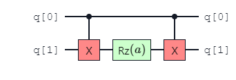
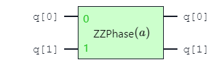
The gate sequence \(CNOT\), \(RZ\), \(CNOT\) can be replaced with the parameterized angle \(ZZ\) gate. This enables a lower number of 2-qubit gates in a quantum circuit, improving performance by decreasing gate errors.
For a narrative on parameterized angle gate usage, please see parameterized 2-qubit gates.
Real-time Classical Computation
The system enables server-side execution of real-time classical compute functions. The control system enables logical expressions on classical registers and conditional operations on qubits. A co-located low-latency, high-performance classical compute environment enables execution of user-defined table-driven or algorithmic QEC (Quantum Error Correction) decoders during the coherence time of qubits [2]. The classical compute environments uses a Wasm runtime, including a Wasm Virtual Machine (WAVM). It offers near-native execution speeds of custom decoders without requiring full-system modification. This environment is sand-boxed to protect against untrusted user code submitted for execution. The classical compute environment offers users 16 GB RAM and leverages an Intel Kabylake processor, however parallelization is not possible with the Wasm runtime. Wasm execution requires network call from the control system to the classical compute environment. A document on real-time QEC decoding is available here.