Transform singular values with QSVT
Download Notebook - qsvt.ipynb
Build a block encoding of a complex matrix, choose a polynomial, and check the resulting quantum singular value transformation (QSVT) against a classical singular-value decomposition. The example uses guppy.
Run this notebook from a source checkout with the development dependencies installed. The repository default is little endian.
1. Encode a complex matrix
Use the two-qubit operator
This matrix is not Hermitian. Its adjoint is obtained by conjugating the coefficients, since each Pauli string is Hermitian. QSVT needs block encodings of both \(A/\lambda\) and \(A^\dagger/\lambda\).
def ham_2q() -> zqp.ComplexTermSum:
    return zqp.ComplexTermSum.from_str("(0.5, Z0 X1), (0.1j, X0 Z1), (0.3j, X0 X1)")

def ham_2q_conj() -> zqp.ComplexTermSum:
    return zqp.ComplexTermSum.from_str("(0.5, Z0 X1), (-0.1j, X0 Z1), (-0.3j, X0 X1)")

ham_op = ham_2q()
ham_op_dagger = ham_2q_conj()
LCUData supplies the term weights and register sizes. Both encodings share PREPARE; conjugating the SELECT coefficients supplies the adjoint:
data = LCUData.from_hamiltonian(ham_op)
data_dagger = LCUData.from_hamiltonian(ham_op_dagger)
prepare = multiplexor_prep(data.amplitudes)

select = build_double_cntrl_select(data)
select_dagger = build_double_cntrl_select(data_dagger)

n_prep_qubits = data.n_prep_qubits
n_state_qubits = data.n_state_qubits

@guppy
@no_type_check
def unprepare(prep: array[qubit, n_prep_qubits]) -> None:
    with dagger:
        prepare(prep)
2. Choose the polynomial
Approximate the bounded, even function
ChebyshevPolynomial computes the approximation; QSPAngleFinder finds its phase sequence in the reflection convention used by QSVT. The phase values are in half-turns.
def target_fun(x):
    """Target function."""
    return np.cos(5 * x) / 2


# Since the function is even, we select an even degree
d_phi = 12
d_cheb = d_phi

target_fun_cheb = ChebyshevPolynomial(target_fun, d_cheb)
qsp_optimizer = QSPAngleFinder(
    d_phi=d_phi, target_polynomial=target_fun_cheb
)

phases = list(qsp_optimizer.phi)
3. Build a classical reference
Write \(A/\lambda=U\Sigma V^\dagger\). For this even polynomial, QSVT acts on the right singular vectors:
For an odd polynomial the corresponding expression is \(U\,p(\Sigma)\,V^\dagger\). The function below handles both cases. We compare against the fitted polynomial, separating circuit accuracy from approximation error.
poly_cos_np = np.polynomial.chebyshev.cheb2poly(qsp_optimizer.target_polynomial.coeffs)
poly_cos_np = Polynomial(poly_cos_np)

actual_hamiltonian = ham_op.to_sparse_matrix().toarray()
actual_hamiltonian_normalized = actual_hamiltonian / data.l1_norm
scipy_qsvt_matrix = scipy_qsvt(actual_hamiltonian_normalized, poly_cos_np)
4. Apply QSVT
Pass the two LCUs and the phase sequence to QSVT. The circuit borrows a preparation register, one signal qubit, and the system register. Initialize the preparation and signal qubits to zero.
@guppy
def qsvt_circ(
    prep_qreg: array[qubit, n_prep_qubits],
    signal_qreg: array[qubit, 1],
    select_qreg: array[qubit, n_state_qubits],
) -> None:
    QSVT(LCU(prepare, select, unprepare),
         LCU(prepare, select_dagger, unprepare),
         comptime(phases)).compose(signal_qreg[0], prep_qreg, select_qreg)
5. Check the encoded block
Project both auxiliary registers onto zero:
get_unitary_projected preserves the block’s scale. The assertion allows an overall global phase and checks the full complex matrix.
post_selection = {
    "prep_qreg": [False for _ in range(n_prep_qubits)],
    "signal": [False],
}

guppy_h = get_unitary_projected(
    qsvt_circ, n_state_qubits, post_selection, endianness=Endianness.LITTLE
)

guppy_h
array([[-2.28558195e-02-2.50045187e-16j,  9.53240766e-16+1.38472763e-01j,
         1.11956617e-15-9.15747495e-17j,  4.51408010e-16+1.01841715e-15j],
       [-1.40232023e-15-1.38472763e-01j, -2.28558195e-02-7.11255119e-16j,
        -9.81654971e-17-1.40506612e-15j,  1.03182541e-15+1.75041488e-16j],
       [-8.90402979e-16-3.10134409e-17j,  2.55095953e-16-1.24459441e-15j,
        -2.28558195e-02-2.49920805e-16j,  1.30825595e-15+1.38472763e-01j],
       [ 1.76636366e-16+7.97034842e-16j, -9.78516939e-16-1.40584214e-16j,
        -1.49882807e-15-1.38472763e-01j, -2.28558195e-02-5.06450891e-16j]])
scipy_qsvt_matrix
array([[2.28556101e-02+0.j       , 0.00000000e+00-0.1384732j,
        0.00000000e+00+0.j       , 0.00000000e+00+0.j       ],
       [0.00000000e+00+0.1384732j, 2.28556101e-02+0.j       ,
        0.00000000e+00+0.j       , 0.00000000e+00+0.j       ],
       [0.00000000e+00+0.j       , 0.00000000e+00+0.j       ,
        2.28556101e-02+0.j       , 6.93889390e-18-0.1384732j],
       [0.00000000e+00+0.j       , 0.00000000e+00+0.j       ,
        0.00000000e+00+0.1384732j, 2.28556101e-02+0.j       ]])
assert_allclose_ignorephase(guppy_h, scipy_qsvt_matrix, threshold=1e-3)
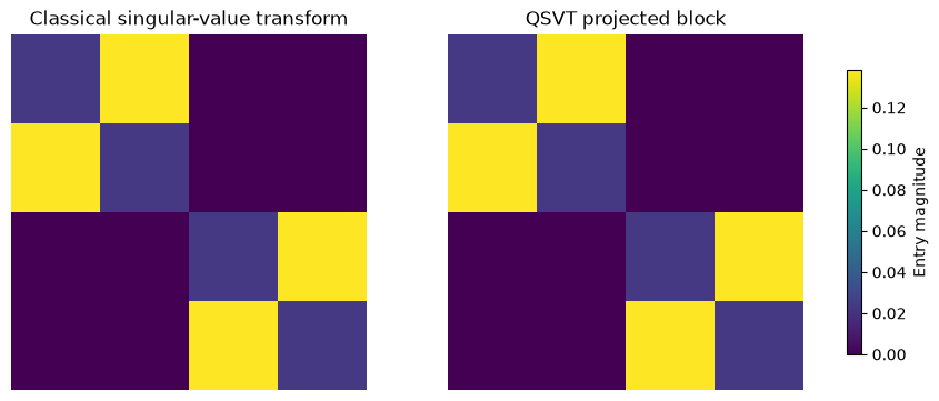
Compare matrix magnitudes
The shared color scale makes the classical and simulated blocks directly comparable. The numerical assertion above also checks their phases, which a magnitude plot cannot show.
import matplotlib.pyplot as plt

fig, axes = plt.subplots(1, 2, figsize=(9, 3.5), layout="constrained")

vmax = max(np.abs(scipy_qsvt_matrix).max(), np.abs(guppy_h).max())
axes[0].imshow(np.abs(scipy_qsvt_matrix), cmap='viridis', vmin=0, vmax=vmax)
axes[0].set_title('Classical singular-value transform')
axes[0].axis('off')

plot = axes[1].imshow(np.abs(guppy_h), cmap='viridis', vmin=0, vmax=vmax)
axes[1].set_title('QSVT projected block')
axes[1].axis('off')

fig.colorbar(plot, ax=axes, label="Entry magnitude", shrink=0.8)
plt.show()