Phase estimation

Phase estimation over different register shapes

Canonical phase estimation is a practical example of the same generic-register pattern. Its essential interface is:

\[ U|\psi\rangle=e^{2\pi i\phi}|\psi\rangle, \qquad \mathrm{QPE}(U,|\psi\rangle)\longrightarrow|\widetilde{\phi}\rangle|\psi\rangle. \]

For three phase qubits, controlled powers imprint the eigenphase before an inverse QFT converts it into a binary estimate:

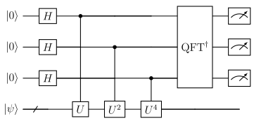
Prepare the Hadamards before calling qpe; the function applies the controlled powers and inverse QFT. A register wire may represent several qubits.

from guppylang import guppy
from guppylang.std.builtins import Function, array, nat
from guppylang.std.quantum import qubit


@guppy
def qpe[n_phase: nat, UnitaryRegs](
    phase_qreg: array[qubit, n_phase],
    unitary_qregs: UnitaryRegs,
    power_oracle: Function[[qubit, UnitaryRegs, int], None],
) -> None:
    ...

• qpe implements phase estimation without inspecting unitary_registers.

• UnitaryRegs describes the complete register shape needed by the selected unitary implementation.

• The same UnitaryRegs appears in the register argument and the oracle signature, so Guppy checks that they are compatible.

• Switching algorithms changes the registers and power oracle, not qpe.

Connect Pauli exponentials to QPE

For Trotterized QPE, each controlled \(U\) box in the circuit above is one controlled Trotter step. That step is built from the controlled Pauli exponentials described in Trotterized Hamiltonian simulation.

For \(H=\sum_j h_jP_j\), one requested power repeats the complete controlled product formula. The phase qubit controls every Pauli exponential:

Here \(p\) is the integer supplied by QPE and \(\delta\) is time_step in the library convention used below.

from guppylang import guppy
from guppylang.std.builtins import array
from guppylang.std.quantum import qubit
from guppyalgos.algorithms.time_evolution.trotter import cntrl_trotter_first_order

import zixy.qubit.pauli as zqp

hamiltonian = zqp.RealTermSum.from_str(
    "(-0.5, Z0 X1), (-0.1, X0 Z1), (-0.2, Y0 Y1)"
)
n_state_qubits = len(hamiltonian.qubits)
cntrl_trotter_step = cntrl_trotter_first_order(hamiltonian, n_state_qubits)
time_step = 0.1


@guppy
def trotter_power_oracle(
    control: qubit,
    state_qreg: array[qubit, n_state_qubits],
    power: int,
) -> None:
    for _ in range(power):
        cntrl_trotter_step(control, state_qreg, time_step)

• A power of \(2^k\) repeats the step \(2^k\) times under the same phase-qubit control.

• Pass this oracle to qpe(phase_qreg, state_qreg, trotter_power_oracle) after preparing the phase superposition and the target state.

• The library’s dimensionless time_step convention gives \(U_{\mathrm{step}}\approx e^{-i\pi\,\mathrm{time\_step}\,H/2}\). Keep that scaling when converting phases to energies.

• Each controlled Pauli exponential uses basis changes, a parity ladder, and a controlled rotation. The outer QPE circuit can therefore stay the same while the Hamiltonian or gate decomposition changes.

Qubitization needs both a PREPARE register and the target registers used by its block encoding. They can be grouped into one generic register value:

One controlled walk expands into the operations used on the block-encoding page. PREPARE and UNPREPARE are unconditional; SELECT and the reflection carry the QPE control. When \(c=0\), PREPARE and UNPREPARE cancel:

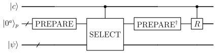
The power oracle repeats this complete controlled walk \(p\) times.

@guppy.struct
class QubitizationRegs[n_prepare: nat, TargetRegs]:
    prep_qreg: array[qubit, n_prepare]
    target_qregs: TargetRegs


@guppy
def qubitization_power_oracle[n_prepare: nat, TargetRegs](
    control: qubit,
    qregs: QubitizationRegs[n_prepare, TargetRegs],
    power: int,
) -> None:
    for _ in range(power):
        cntrl_walk(control, qregs.prep_qreg, qregs.target_qregs)

• Here, UnitaryRegs becomes QubitizationRegs[n_prepare, TargetRegs].

• cntrl_walk applies one controlled qubitization step; the power oracle repeats it exactly as the Trotter oracle repeats its controlled step.

• TargetRegs can itself be a qubit array, tuple, or Guppy struct, provided the controlled walk and power oracle accept the same type.

This keeps phase estimation independent of how the simulated unitary arranges its state and work registers. See the canonical phase-estimation notebook for array and struct examples, and the Trotterized phase-estimation notebook for complete powered-Trotter oracles.

Qubitized phase estimation

Using the quantum walk constructed in Block encoding, phase estimation can estimate the walk’s eigenphase and convert it back to an energy. Its target is the combined preparation and system registers, represented by QubitizationRegs in the library.

For three phase qubits, the structure is:

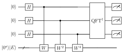
• Prepare the phase register with Hadamards before calling qpe. The library’s qpe applies controlled powers and the inverse QFT.

• qubitized_power_oracle repeats the controlled walk for the requested integer power. With \(m\) phase qubits, this uses \(2^m-1\) walk steps.

• A Hamiltonian eigenstate with a zero preparation register generally overlaps both walk eigenstates. The two conjugate phases encode the same energy.

• Energy-sampling probabilities depend on the input’s eigenstate overlaps; QPE does not itself prepare the ground state.

Decode the sampled phase

The repository’s binary_fraction helper expresses the phase in half-turns: \(U|\omega\rangle=e^{i\pi\phi}|\omega\rangle\), with \(0\leq\phi<2\). The conversion from \(\phi\) depends on the power oracle.

Trotterized Hamiltonian simulation

For the repository’s time-evolution convention,

\[ U(t)=e^{-i\pi tH/2},\qquad U(t)|E\rangle=e^{-i\pi tE/2}|E\rangle. \]

Comparing the exponent with \(e^{i\pi\phi}\) gives

\[ \phi=-\frac{tE}{2}\pmod 2, \qquad E=-\frac{2(\phi+2k)}{t}. \]

The integer \(k\) selects the correct phase-wrapping branch. The helper phase_to_energy_qpe(phi, total_time, phase_wraps=k) performs this conversion.

For example, the phase-estimation demo uses \(H=(X+Z)/2\), its ground energy \(E=-1/\sqrt2\), and \(t=1\). The exact phase is \(1/(2\sqrt2)\approx0.3536\). Six phase qubits resolve the nearby bin \(11/32\), giving \(E\approx-0.6875\).

Qubitized phase estimation

For the qubitization walk \(W\), the sampled phase instead satisfies

\[ E=-\lambda\cos(\pi\phi), \qquad \phi\ \text{and}\ 2-\phi\ \text{give the same }E. \]

The helper phase_to_energy_qubitized_qpe(phi, data.l1_norm) implements this conversion. For example, \(H=(X+Z)/2\) has normalization \(\lambda=1\). Its positive eigenvalue \(1/\sqrt{2}\) produces half-turn phases \(3/4\) and \(5/4\), both exactly representable with three phase qubits.

The qubitized phase-estimation notebook demonstrates the larger Hamiltonian

\[ H=0.5Z_0X_1Y_2+0.1X_0Z_1Z_2+0.2Y_0Y_1X_2+0.3X_0X_1Y_2. \]

It combines LCUData, build_cntrl_unary_iteration_select, QubitizationCntrl, and qpe, then compares sampled energies with exact diagonalization. Its five-qubit phase register has grid spacing \(2/2^5\). Exact eigenstate preparation is used there as a small-system validation tool.