Block encoding

A block encoding places a matrix inside a larger unitary. This lets us use a Hamiltonian in a quantum circuit without requiring the Hamiltonian itself to be a gate. The examples below build on each other; a runnable version with matrix checks is in the block-encoding demo.

LCU: a weighted sum of unitaries

LCU stands for linear combination of unitaries. It represents an operator as a weighted sum of unitary terms,

\[ H=\sum_j a_jU_j. \]

Pauli strings are unitary, so a Pauli Hamiltonian has this form directly. PREPARE loads the term weights, SELECT applies the chosen \(U_j\), and UNPREPARE reverses the preparation:

\[ H=\sum_j a_jU_j,\qquad \lambda=\sum_j|a_j|,\qquad \langle0^a|B|0^a\rangle=H/\lambda. \]

The block encoding \(B\) is the following circuit:

LCUData calculates the amplitudes \(\sqrt{|a_j|/\lambda}\) and the SELECT builder includes each coefficient’s phase. LCU composes the three routines.

Two terms

Take \(H=0.6X+0.4Y\), so \(\lambda=1\). One preparation qubit is enough:

\[\begin{split} \begin{aligned} \mathrm{PREPARE}|0\rangle&=\sqrt{0.6}|0\rangle+\sqrt{0.4}|1\rangle,\\ \mathrm{SELECT}&=|0\rangle\langle0|\otimes X+|1\rangle\langle1|\otimes Y. \end{aligned} \end{split}\]

Choose \(\theta=2\arccos\sqrt{0.6}\) in radians. PREPARE is \(R_y(\theta)\), and UNPREPARE is \(R_y(-\theta)\):

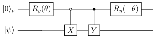
The code below uses multiplexor_prep for the rotation and writes the two SELECT branches explicitly.

import zixy.qubit.pauli as zqp
from guppylang import guppy
from guppylang.std.builtins import array, comptime, dagger
from guppylang.std.quantum import cx, cy, qubit, toffoli, x

from guppyalgos.algorithms.block_encoding.lcu import LCU, LCUData
from guppyalgos.algorithms.state_preparation import multiplexor_prep

hamiltonian = zqp.RealTermSum.from_str("(0.6, X0), (0.4, Y0)", 1)
data = LCUData.from_hamiltonian(hamiltonian)
prepare = multiplexor_prep(data.amplitudes)


@guppy
def select(prep_qreg: array[qubit, 1], qreg: array[qubit, 1]) -> None:
    # Open control: apply X when the preparation qubit is |0>.
    x(prep_qreg[0])
    cx(prep_qreg[0], qreg[0])
    x(prep_qreg[0])

    # Closed control: apply Y when the preparation qubit is |1>.
    cy(prep_qreg[0], qreg[0])


@guppy
def unprepare(prep_qreg: array[qubit, 1]) -> None:
    with dagger:
        prepare(prep_qreg)


@guppy
def block_encode(prep_qreg: array[qubit, 1], qreg: array[qubit, 1]) -> None:
    LCU(prepare, select, unprepare).compose(prep_qreg, qreg)

Start prep_qreg at zero. Post-selecting it on zero exposes the block \(H\); leave it coherent when the encoding is part of a larger algorithm.

Qubitization

A walk step applies the block encoding followed by a reflection on the preparation register:

\[ W=RB,\qquad R=I-2|0^a\rangle\langle0^a|. \]

• \(B\) contains \(H/\lambda\) in its all-zero preparation block.

• \(R\) changes the sign of that preparation state.

• Their product turns each eigenvalue of \(H\) into a phase that QPE can read.

For the two-term example, PREPARE is a Y rotation with \(\theta=2\arccos\sqrt{0.6}\) in radians. The open control selects X at address zero; the filled control selects Y at address one.

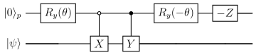
multiplexor_prep supplies the preparation above; Reflection[1, 0] supplies the one-qubit reflection. Qubitization puts them together:

from guppyalgos.algorithms.block_encoding.qubitization import Qubitization
from guppyalgos.primitives.subroutines.reflection import Reflection
from guppyalgos.primitives.gate_decompositions.cnx.cnx import cnx


@guppy
def walk(prep_qreg: array[qubit, 1], qreg: array[qubit, 1]) -> None:
    Qubitization(
        LCU(prepare, select, unprepare), Reflection[1, 0](cnx)
    ).compose(prep_qreg, qreg)

Walk powers

Let \(|E\rangle\) be an eigenstate of \(H\) and put \(x=E/\lambda\). In the eigenbasis of \(H\), the walk separates into two-dimensional invariant subspaces. One basis vector has the preparation register in \(|0^a\rangle\); the other is its orthogonal partner. On this subspace,

\[\begin{split} \begin{aligned} B_E&=\begin{pmatrix}x&\sqrt{1-x^2}\\\sqrt{1-x^2}&-x\end{pmatrix},\\[6pt] W_E&=\begin{pmatrix}-1&0\\0&1\end{pmatrix}B_E\\[6pt] &=\begin{pmatrix}-x&-\sqrt{1-x^2}\\\sqrt{1-x^2}&-x\end{pmatrix}. \end{aligned} \end{split}\]

Writing \(\vartheta_E=\arccos(-x)\) gives

\[\begin{split} W_E= \begin{pmatrix} \cos\vartheta_E&-\sin\vartheta_E\\ \sin\vartheta_E&\cos\vartheta_E \end{pmatrix} =R_y(2\vartheta_E). \end{split}\]

The walk is therefore a Y rotation on each eigenvalue subspace. Its two eigenphases are \(e^{\pm i\vartheta_E}\), and either phase recovers the energy through \(E=-\lambda\cos\vartheta_E\). This is the link between the block encoding and qubitized phase estimation.

Repeated steps encode Chebyshev polynomials. In particular, \(\langle0^a|W^2|0^a\rangle=2(H/\lambda)^2-I\):

@guppy
def walk_squared(prep_qreg: array[qubit, 1], qreg: array[qubit, 1]) -> None:
    Qubitization(
        LCU(prepare, select, unprepare), Reflection[1, 0](cnx)
    ).power(prep_qreg, qreg, 2)

Controlled walks

QubitizationCntrl adds an external control to SELECT and the reflection. PREPARE and UNPREPARE remain unconditional and cancel when the control is zero.

from guppyalgos.algorithms.block_encoding.lcu import (
    LCUCntrl, build_cntrl_single_cntrl_select,
)
from guppyalgos.algorithms.block_encoding.qubitization import QubitizationCntrl
from guppyalgos.primitives.subroutines.reflection import ReflectionCntrl

controlled_select = build_cntrl_single_cntrl_select(data)


@guppy
def controlled_walk(
    control: qubit, prep_qreg: array[qubit, 1], qreg: array[qubit, 1],
) -> None:
    QubitizationCntrl(
        LCUCntrl(prepare, controlled_select, unprepare), ReflectionCntrl[1](cnx)
    ).compose(control, prep_qreg, qreg)

Use this controlled step in Phase estimation.

SELECT and unary iteration

SELECT applies an operation indexed by a quantum address:

\[ \mathrm{SELECT}|j\rangle|\psi\rangle=|j\rangle U_j|\psi\rangle. \]

For a superposition, each address receives its own operation. The address is preserved and can become entangled with the target.

The four-term circuit below shows the basic pattern. A direct implementation would give every \(U_j\) two controls. Unary iteration computes one address flag and updates it as the little-endian address advances.

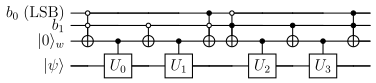
The example below supplies eight arbitrary Pauli operations. The builder adds the address cascade around their controlled forms:

from guppyalgos.algorithms.select import build_select_unary_from_data
from guppyalgos.primitives.gate_decompositions.and_op import (
    temp_and_compute, temp_and_uncompute,
)
from guppyalgos.primitives.pauli import pauli_to_cntrl_gate

terms = [
    zqp.String.from_str(label, 2)
    for label in (
        "X0", "Y0", "Z0", "X1", "Y1", "Z1", "X0 X1", "Z0 Y1",
    )
]

unary_select_toffoli = build_select_unary_from_data(
    terms,
    lambda term: pauli_to_cntrl_gate(term, 2),
    comp_and_op=toffoli,
    uncomp_and_op=toffoli,
)

unary_select_temporary_and = build_select_unary_from_data(
    terms,
    lambda term: pauli_to_cntrl_gate(term, 2),
    comp_and_op=temp_and_compute,
    uncomp_and_op=temp_and_uncompute,
)


@guppy
def select_example(index_qreg: array[qubit, 3], qreg: array[qubit, 2]) -> None:
    unary_select_toffoli(index_qreg, qreg)

Compute	Uncompute	Behavior
toffoli	toffoli	Fully unitary cascade shown above.
temp_and_compute	temp_and_uncompute	Four-T temporary AND compute with measurement-based uncomputation.

Both choices implement the same SELECT. The temporary-AND version trades mid-circuit measurement and feed-forward for a lower T cost. The builder also accepts other compatible three-qubit compute and uncompute functions. In every case, the work flags are cleared before SELECT returns.

This construction follows the unary-iteration approach introduced in Babbush et al., Physical Review X 8, 041015 (2018). For a Pauli LCU, build_unary_iteration_select(data) builds the term operations directly from LCUData.

QROM and fanout

QROM uses the same unary-iteration machinery under the hood. It computes the same address flag and updates it with the same adjacent-AND cascade. Only the controlled operation changes: SELECT applies \(U_j\), while QROM fans the active flag out to the one-bits of a classical word and XORs them into a data register:

\[ \mathrm{QROM}|j\rangle|y\rangle=|j\rangle|y\oplus d_j\rangle, \qquad U_j=\bigotimes_k X_k^{d_{j,k}}. \]

Each one-bit in the word adds a controlled X. For the word [True, False, True], the active address flag controls these two gates:

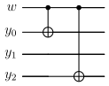
The table is fixed when the circuit is built. Each row below lists bits by qubit index; the repository default is little endian.

from guppyalgos.algorithms.select.qrom import qrom_unary_iteration
from guppyalgos.primitives.subroutines.fanout import (
    fanout_basic, fanout_log, fanout_measurement_parity,
)

words = [
    [True, False, True],
    [False, True, True],
    [True, True, False],
    [True, True, True],
]
lookup = qrom_unary_iteration(words, fanout_op=fanout_basic)


@guppy
def qrom_example(index_qreg: array[qubit, 2], data_qreg: array[qubit, 3]) -> None:
    lookup(index_qreg, data_qreg)

An initially zero data register receives the selected word. Calling the lookup twice restores the original data, provided the address is unchanged.

Choose the fanout

Change fanout_op to choose how the active flag reaches the selected data qubits. The table and the QROM call signature stay the same:

lookup_log = qrom_unary_iteration(words, fanout_op=fanout_log)
lookup_measurement = qrom_unary_iteration(words, fanout_op=fanout_measurement_parity)


@guppy
def qrom_log_example(index_qreg: array[qubit, 2], data_qreg: array[qubit, 3]) -> None:
    lookup_log(index_qreg, data_qreg)


@guppy
def qrom_measurement_example(
    index_qreg: array[qubit, 2], data_qreg: array[qubit, 3],
) -> None:
    lookup_measurement(index_qreg, data_qreg)

Fanout	Implementation
fanout_basic	Sequential CNOTs from the flag to each selected bit.
fanout_log	A logarithmic-depth CNOT ladder.
fanout_measurement_parity	Measurement-assisted parity with feed-forward; uses extra ancillas for four or more selected bits.

All three work on arbitrary data-register states. The small table above has two or three selected bits per word; larger words expose the different depth and workspace costs. The current fanout_log requires at least one selected bit per word. Use fanout_from_data_fn when a custom register structure also needs a different adapter.

See the QROM notebook for a complete data-loading example.

QSVT

QSVT alternates a block encoding and its adjoint with phase rotations to transform its singular values. The alternating sequence needs both \(B\) and \(B^\dagger\): moving forward through one phase step uses the LCU encoding, and the next step reverses it with the adjoint. This preserves the two-dimensional signal subspaces in which the polynomial transformation is constructed.

For the Hermitian example above, \(B^\dagger=B\), so both QSVT arguments can use the same LCU. The three half-turn phases [0.5, 0.5, 0.5] encode the odd cubic polynomial

\[ p(x)=\frac{x-2x^3}{\sqrt2}, \qquad p(H/\lambda)=\frac{H/\lambda-2(H/\lambda)^3}{\sqrt2}. \]

Unlike a simple rescaling, this changes different singular values by different amounts while preserving the sign of an odd input spectrum.

from guppyalgos.algorithms.block_encoding.qsvt import QSVT

phases = [0.5, 0.5, 0.5]


@guppy
def polynomial(
    signal: qubit, prep_qreg: array[qubit, 1], qreg: array[qubit, 1],
) -> None:
    QSVT(
        LCU(prepare, select, unprepare),
        LCU(prepare, select, unprepare),
        comptime(phases),
    ).compose(signal, prep_qreg, qreg)

Project the signal and preparation qubits onto zero to obtain the polynomial block. For a general LCU whose block encoding is not Hermitian, the second argument must implement the actual reversed and adjointed circuit \(B^\dagger\) rather than reusing \(B\).

The QSVT notebook shows how to find phases for a chosen polynomial using ChebyshevPolynomial and QSPAngleFinder.