Hamiltonian simulation: build, evolve, measure

Download Notebook - ham_sim_trotter_demo.ipynb

• Build an evolution circuit from a Hamiltonian written as Pauli terms.

• Measure observables directly, with expectation values and uncertainties calculated by the library.

• Swap circuit components: replace the underlying rotation implementation while keeping the evolution and measurement interfaces.

This demo follows one two-qubit system from preparation to measured dynamics. The same components can be reused for other Hamiltonians and input states.

What you want to do	Library component
Build a Trotter step	trotter_first_order
Evolve for several steps	ham_sim_trotter
Measure a Pauli observable	make_direct_measure_pauli_simple
Calculate a mean and uncertainty	estimate_pauli_observable_expectation_from_bitstrings
Replace the rotation implementation	The step factory’s rz_method argument

• Each section introduces one part of the workflow, with runnable code and saved results.

• Run from a source checkout with development dependencies installed. The repository default is little endian.

Show code cell source

Hide code cell source

from math import ceil, log2

import numpy as np
import pandas as pd
import zixy.qubit.pauli as zqp
from scipy.linalg import expm
from matplotlib import pyplot as plt
from selene_sim import QuantumReplay, Quest
from guppylang import guppy
from guppylang.std.builtins import array
from guppylang.std.quantum import qubit, h
from guppyalgos.utils import qarray, transversal
from guppyalgos.algorithms.time_evolution.trotter import ham_sim_trotter, trotter_first_order
from guppyalgos.primitives.measurement import (
    make_direct_measure_pauli_simple,
    estimate_pauli_observable_expectation_from_bitstrings,
)

1. Build an evolution circuit

Choose a Hamiltonian

• Describe the system as a weighted sum of Pauli strings, \(H=\sum_j a_jP_j\).

• This example uses two qubits and four terms:

\[ H=-0.5Z_0X_1-0.1X_0Z_1-0.2Y_0Y_1-0.3X_0X_1. \]

• Change the coefficients and Pauli strings to describe a different system.

hamiltonian = zqp.RealTermSum.from_str(
    "(-0.5, Z0 X1), (-0.1, X0 Z1), (-0.2, Y0 Y1), (-0.3, X0 X1)", 2,
)
n_qubits = 2
time_step = 0.2
n_shots = 1024

Compose the simulation

• trotter_first_order builds one step from the Hamiltonian.

• ham_sim_trotter repeats it. Five steps of size \(0.2\) give total time \(t=1\).

\[ U_r(t)=\left[\prod_j e^{-i\pi\Delta t\,a_jP_j/2}\right]^r, \qquad t=r\Delta t. \]

trotter_step = trotter_first_order(hamiltonian, n_qubits)
simulation = ham_sim_trotter(trotter_step, n_steps=5, time_step=time_step, n_state_qubits=n_qubits)

Choose the input state

• qreg holds the two system qubits.

• transversal(h, qreg) prepares \(|+\rangle^{\otimes2}\); simulation(qreg) evolves it.

• Replace the preparation gates to study a different initial state.

@guppy
def prepare(qreg: array[qubit, 2]) -> None:
    transversal(h, qreg)
    simulation(qreg)

2. Measure an observable

Choose the measurement basis

• make_direct_measure_pauli_simple builds the basis changes and measurements for a Pauli string.

• Use the same interface for \(X\), \(Y\), \(Z\), or products such as \(Z_0X_1\).

• The small runner below prepares a fresh state for each shot and collects the library’s measurement output.

def sample_direct(
    preparation, pauli, seed=7, extra_qubits=0, shots=n_shots, simulator=None,
):
    measurement = make_direct_measure_pauli_simple(pauli, n_qubits)

    @guppy
    def experiment() -> None:
        qreg = qarray(n_qubits)
        preparation(qreg)
        measurement(qreg)

    emulator = experiment.emulator(n_qubits + extra_qubits).with_seed(seed)
    if simulator is not None:
        emulator = emulator.with_simulator(simulator)
    result = emulator.with_shots(shots).run()
    return [shot["bitstring"][0] for shot in result.collated_shots()]

Turn shots into an expectation value

• Ask for \(\langle Z_0\rangle\) and collect 1,024 shots.

• The built-in estimator handles parity, averaging, and standard error:

\[ \widehat{\langle P\rangle}=\frac{N_+-N_-}{N}, \qquad \mathrm{SE}=\sqrt{\frac{1-\widehat{\langle P\rangle}^2}{N}}. \]

• A Pauli expectation lies in \([-1,1]\). For \(Z_0\), the corresponding probability is \(\Pr(q_0=1)=(1-\langle Z_0\rangle)/2\).

observable = zqp.RealTermSum.from_str("Z0", n_qubits)
pauli = zqp.String.from_str("Z0", n_qubits)
samples = sample_direct(prepare, pauli)
estimate = estimate_pauli_observable_expectation_from_bitstrings(observable, {str(pauli): samples})
print(pd.DataFrame([{
    "Observable": "Z0", "Expectation": estimate.expectation,
    "Standard error": estimate.standard_error, "Shots": n_shots,
}]).to_string(index=False, float_format=lambda value: f"{value:.4f}"))

Observable  Expectation  Standard error  Shots
        Z0       0.3633          0.0291   1024

3. See the dynamics

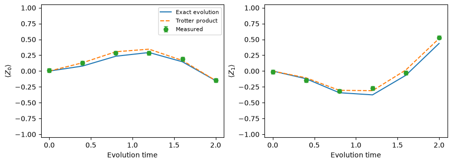
• Increase the number of steps to follow the state over time.

• Measure \(\langle Z_0\rangle\) and \(\langle Z_1\rangle\) using the same measurement runner.

• Here \(\Delta t=0.2\) stays fixed, so more steps mean a longer evolution. To improve the Trotter approximation at a fixed time, increase the step count while reducing \(\Delta t=t/r\).

Set up a reference

• Exact evolution uses \(e^{-i\pi tH/2}\).

• The Trotter reference multiplies the same Pauli rotations as the circuit, with later gates on the left.

• Keeping both references lets us distinguish approximation error from measurement noise.

Show code cell source

Hide code cell source

initial_state = np.ones(2**n_qubits) / np.sqrt(2**n_qubits)
h_matrix = np.asarray(hamiltonian.to_sparse_matrix(True).todense())
step_matrix = np.eye(2**n_qubits, dtype=complex)
for term in hamiltonian.to_terms():
    matrix = float(term.coeff) * np.asarray(term.string.to_sparse_matrix(True).todense())
    step_matrix = expm(-0.5j * np.pi * time_step * matrix) @ step_matrix


def reference_mean(state, operator):
    matrix = np.asarray(operator.to_sparse_matrix(True).todense())
    return float(np.vdot(state, matrix @ state).real)

Reuse the circuit and measurement builders

• Build an evolution for each time point.

• Pass each observable to the same sample_direct runner.

• Check the measured values against the Trotter reference, allowing for finite-shot noise.

Show code cell source

Hide code cell source

step_counts = [0, 2, 4, 6, 8, 10]
rows = []
for steps in step_counts:
    evolve = ham_sim_trotter(trotter_step, steps, time_step, n_qubits)

    @guppy
    def prepare_at_time(qreg: array[qubit, 2]) -> None:
        transversal(h, qreg)
        evolve(qreg)

    time = steps * time_step
    exact_state = expm(-0.5j * np.pi * time * h_matrix) @ initial_state
    trotter_state = np.linalg.matrix_power(step_matrix, steps) @ initial_state
    for index in range(n_qubits):
        label = f"Z{index}"
        operator = zqp.RealTermSum.from_str(label, n_qubits)
        pauli = zqp.String.from_str(label, n_qubits)
        samples = sample_direct(prepare_at_time, pauli, seed=100 + 2 * steps + index)
        stats = estimate_pauli_observable_expectation_from_bitstrings(operator, {str(pauli): samples})
        reference = reference_mean(trotter_state, operator)
        assert abs(stats.expectation - reference) < 5 / np.sqrt(n_shots)
        rows.append({"Time": time, "Observable": label, "Sampled": stats.expectation,
                     "SE": stats.standard_error, "Trotter": reference,
                     "Exact": reference_mean(exact_state, operator)})
dynamics = pd.DataFrame(rows)

Read the result

• Dots and error bars: sampled expectations with one standard error.

• Dashed curves: the implemented Trotter product.

• Solid curves: exact Hamiltonian evolution.

• The gap between the curves is Trotter error; fluctuations around the dashed curve are sampling noise.

Show code cell source

Hide code cell source

fig, axes = plt.subplots(1, 2, figsize=(9, 3.2), layout="constrained")
for index, axis in enumerate(axes):
    values = dynamics[dynamics["Observable"] == f"Z{index}"]
    axis.plot(values["Time"], values["Exact"], label="Exact evolution")
    axis.plot(values["Time"], values["Trotter"], "--", label="Trotter product")
    axis.errorbar(values["Time"], values["Sampled"], yerr=values["SE"], fmt="o", capsize=3, label="Measured")
    axis.set(xlabel="Evolution time", ylabel=rf"$\langle Z_{index}\rangle$", ylim=(-1.05, 1.05))
axes[0].legend(fontsize=8)
plt.show()

4. Swap the rotation implementation

• Pass a different rz_method to trotter_first_order to change the rotations inside each Pauli exponential.

• ham_sim_trotter and the measurement runner keep the same interfaces.

• Here we use comparator_based_rz_cascade, which implements approximate rotations with measurement feedback.

• epsilon controls individual rotations; it is not a bound on the full simulation error.

from guppyalgos.primitives.rotations import comparator_based_rz_cascade, n_comparator_based_rz_cascade_ancillas

epsilon = 0.1
rus_step = trotter_first_order(
    hamiltonian, n_qubits, rz_method=comparator_based_rz_cascade(epsilon),
)
rus_ancillas = n_comparator_based_rz_cascade_ancillas(epsilon)

Build the RUS evolution circuit

• Use the same Hamiltonian, initial state and time step as above; sample the comparator implementation at step 4.

• Only the rotation implementation changes. The builder returns the preparation circuit for a chosen number of steps.

def make_rus_preparation(steps):
    evolve_rus = ham_sim_trotter(rus_step, steps, time_step, n_qubits)

    @guppy
    def prepare_rus_at_time(qreg: array[qubit, 2]) -> None:
        transversal(h, qreg)
        evolve_rus(qreg)

    return prepare_rus_at_time

Sample the comparator dynamics

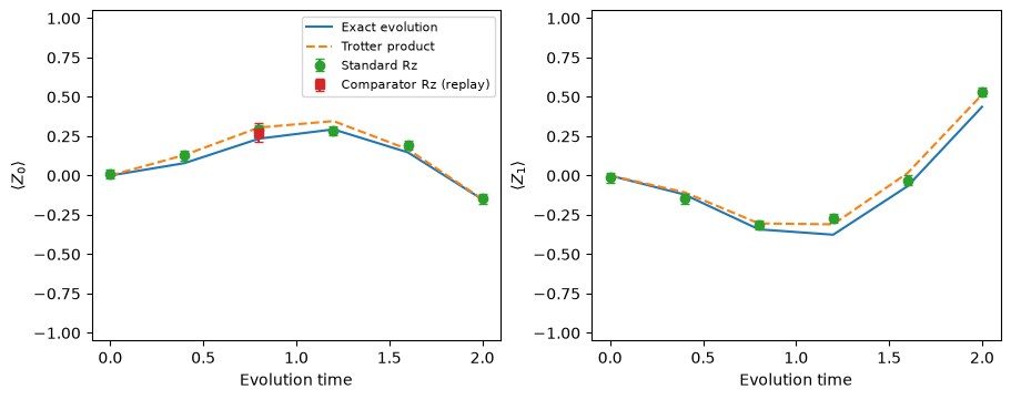
• Use 256 shots at step 4 (\(t=0.8\)).

• Measure only \(Z_0\) for this comparison point.

• QuantumReplay fixes each RUS attempt to immediate success, avoiding repeated probabilistic retries. The underlying Quest simulator still samples the final observables.

rus_steps = 4
rus_shots = 256
n_rus_bits = 1 + ceil(log2(1 / epsilon))
n_rus_rotations = rus_steps * len(hamiltonian)
immediate_success = [False] * (n_rus_rotations * (2 * n_rus_bits - 2))
replay_simulator = QuantumReplay(
    simulator=Quest(random_seed=900 + rus_steps),
    measurements=[immediate_success.copy() for _ in range(rus_shots)],
)

label = "Z0"
samples = sample_direct(
    make_rus_preparation(rus_steps), zqp.String.from_str(label, n_qubits),
    seed=900 + rus_steps, shots=rus_shots, extra_qubits=rus_ancillas,
    simulator=replay_simulator,
)
operator = zqp.RealTermSum.from_str(label, n_qubits)
stats = estimate_pauli_observable_expectation_from_bitstrings(
    operator, {label: samples},
)
rus_dynamics = pd.DataFrame([{
    "Time": rus_steps * time_step, "Observable": label,
    "Sampled": stats.expectation, "SE": stats.standard_error,
}])

Compare \(Z_0\)

• Circles show standard-Rz samples; the square shows the comparator-Rz \(Z_0\) sample.

• Compare the step-4 point with the standard-Rz sample and Trotter reference; exact evolution is also shown.

• Comparator results also include rotation-approximation error; error bars describe sampling uncertainty only.

standard_z0 = dynamics[dynamics["Observable"] == "Z0"]
fig, axis = plt.subplots(figsize=(6, 3.5), layout="constrained")
axis.plot(standard_z0["Time"], standard_z0["Exact"], label="Exact evolution")
axis.plot(standard_z0["Time"], standard_z0["Trotter"], "--", label="Trotter product")
axis.errorbar(standard_z0["Time"], standard_z0["Sampled"],
              yerr=standard_z0["SE"], fmt="o", capsize=3, label="Standard Rz")
axis.errorbar(rus_dynamics["Time"], rus_dynamics["Sampled"],
              yerr=rus_dynamics["SE"], fmt="s", capsize=3,
              label="Comparator Rz (replay)")
axis.set(xlabel="Evolution time", ylabel=r"$\langle Z_0\rangle$", ylim=(-1.05, 1.05))
axis.legend(fontsize=8)
plt.show()

Explore further

• Use the QPE demo to estimate energy eigenvalues with controlled evolution.

• Explore Pauli exponentials to see how the rotation and CX-ladder implementations fit together.