Find QSP and GQSP phases

Download Notebook - qsp_angle_finder.ipynb

Phase synthesis translates a target function into the classical parameters of a quantum signal-processing sequence. This notebook follows two routes: a Chebyshev approximation for QSP, and a Fourier approximation for generalized QSP (GQSP).

Show code cell source

Hide code cell source

import numpy as np
from matplotlib import pyplot as plt

from guppyalgos.utils import ChebyshevPolynomial, QSPAngleFinder
from guppyalgos.utils import FourierPolynomial, GQSPAngleFinder

1. QSP for an exponential filter

On \(x\in[0,1]\), use the Gibbs-like filter \(e^{-\beta x}\). QSP requires a definite parity, so extend it evenly:

\[ f(x)=e^{-\beta|x|},\qquad f(-x)=f(x). \]

This is a filter function, rather than a normalized probability distribution. The helper below can construct even or odd extensions; this example uses the even one.

# Target functions 

def _gibbs_fun(x, beta):
    return np.exp(-beta * x)


def generate_gibbs_fun(beta):
    def fun(x):
        return _gibbs_fun(x, beta)

    return fun


def symmetrize_fun(fun, parity=0):
    if parity == 0:

        def neg_fun(x):
            return fun(-x)

        def pos_fun(x):
            return fun(x)

    if parity == 1:

        def neg_fun(x):
            return -fun(-x)

        def pos_fun(x):
            return fun(x)

    def sfun(x):
        if x < 0:
            return neg_fun(x)
        if x >= 0:
            return pos_fun(x)

    return np.vectorize(sfun)

beta = 2.5

gibbs_fun = generate_gibbs_fun(beta)
sym_gibbs_fun = symmetrize_fun(gibbs_fun, 0)
antisym_gibbs_fun = symmetrize_fun(gibbs_fun, 1)

Approximate the function

ChebyshevPolynomial fits the even extension with a degree-16 polynomial:

\[ p_d(x)=\sum_{k=0}^{d}c_kT_k(x),\qquad d=16. \]

The .error value reports the approximation error. Increasing the degree can improve the fit, at the cost of a longer quantum sequence.

d_phi = 16
d_cheb = d_phi

sym_gibbs_cheb = ChebyshevPolynomial(sym_gibbs_fun, d_cheb)
sym_gibbs_cheb.error

np.float64(0.08752003120788343)

Optimize the phases

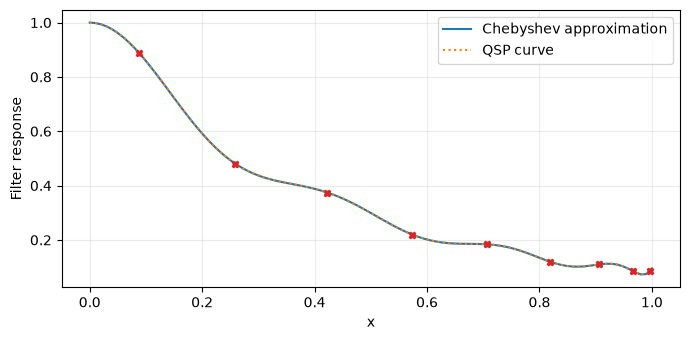
QSPAngleFinder chooses phase factors so that the QSP response approximates \(p_d(x)\). Its .opt_error measures phase-synthesis error, separately from the polynomial approximation error. The plot compares the fitted polynomial with the synthesized response.

qsp_optimizer = QSPAngleFinder(d_phi=d_phi, target_polynomial=sym_gibbs_cheb)
qsp_optimizer.opt_error

np.float64(1.143961726692128e-09)

plt.figure(figsize=(7, 3.5))
x_vals=np.linspace(0, 1, 100)
f_vals = qsp_optimizer(x=x_vals)
plt.plot(x_vals, qsp_optimizer.target_polynomial(x_vals), label="Chebyshev approximation")
plt.plot(x_vals, f_vals, linestyle="dotted", label="QSP curve")
for x_j in qsp_optimizer.x_Chebyshev_roots:
    plt.plot(
        [x_j],
        [qsp_optimizer.target_polynomial(x_j)],
        color="C3",
        marker="X",
        markersize=5,
    )
plt.xlabel("x")
plt.ylabel("Filter response")
plt.grid(alpha=0.25)
plt.tight_layout()
plt.legend()
plt.show()

2. GQSP from a Fourier series

GQSP represents a function of a unitary using a Laurent polynomial:

\[ F(z)=\sum_{k=-20}^{20}c_kz^k,\qquad z=e^{i\pi x}. \]

For the periodic extension of \(e^{-\tau\pi|x|}\) on \([-1,1]\), use

\[ c_k=\frac{\tau\bigl(1-(-1)^k e^{-\pi\tau}\bigr)}{\pi(\tau^2+k^2)}. \]

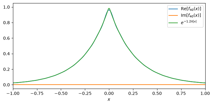
FourierPolynomial stores these coefficients. The first plot shows the truncated series and its target.

tau = 1.2
degree = 40

d_max = degree // 2
d_min = - degree // 2

f_coeffs = {
    k : (tau*(1+((-1)**(k+1))*np.exp(-np.pi*tau)))/(np.pi*(tau**2 + k**2))
    for k in range(d_min, d_max+1)
}

f = FourierPolynomial(f_coeffs, d_max, d_min)

plt.figure(figsize=(7, 3.5))
xax = np.linspace(-1, 1, 200)
plt.plot(xax, f(xax).real, label=rf'Re$[f_{{{degree}}}(x)]$', color='C0')
plt.plot(xax, f(xax).imag, label=rf'Im$[f_{{{degree}}}(x)]$', color='C1')
plt.plot(xax, np.exp(-tau*np.pi*np.abs(xax)), label=rf'$e^{{-{float(tau):.3} \pi |x|}}$', color='C2')
plt.legend()
plt.xlim(-1, 1)
plt.ylim(-0.05,1.05)
plt.xlabel(r'$x$')
plt.tight_layout()

Construct the complementary polynomial

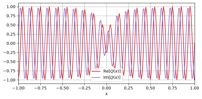
GQSPAngleFinder constructs a second polynomial \(Q\) so that, on the unit circle,

\[ |F(z)|^2+|Q(z)|^2=1. \]

This is the normalization needed to embed the polynomial in a unitary. The construction requires a bounded target; finite-precision arithmetic can leave a small numerical residual.

angle_finder = GQSPAngleFinder(f)

plt.figure(figsize=(7, 3.5))
# Let us plot the complementary function h(x)

q = angle_finder.complementary_polynomial
plt.plot(xax, q(xax).real, label=r'Re$[ Q(x) ]$', color='C3')
plt.plot(xax, q(xax).imag, label=r'Im$[ Q(x) ]$', color='C4')
plt.xlim(-1,1)
plt.xlabel(r'x')
plt.grid()
plt.legend()
plt.tight_layout()
plt.show()

residual = np.max(np.abs(np.abs(f(xax))**2 + np.abs(q(xax))**2 - 1))
print(f"Maximum normalization residual on the grid: {residual:.2e}")

Maximum normalization residual on the grid: 1.63e-13

Retrieve the phase factors

.phase_factors contains the parameters for the GQSP sequence. The preceding residual checks the complementary-polynomial condition; it is not a measure of the original Fourier approximation error.

phase_factors = angle_finder.phase_factors