Binary classification using pytket-qujax

Download this notebook - pytket-qujax-classification.ipynb

See the docs for qujax and pytket-qujax.

from jax import numpy as jnp, random, vmap, value_and_grad, jit
from pytket import Circuit
from pytket.circuit.display import render_circuit_jupyter
from pytket.extensions.qujax.qujax_convert import tk_to_qujax
import matplotlib.pyplot as plt

Define the classification task

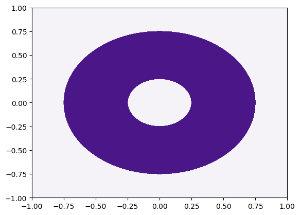
We’ll try and learn a donut binary classification function (i.e. a bivariate coordinate is labelled 1 if it is inside the donut and 0 if it is outside)

inner_rad = 0.25
outer_rad = 0.75

def classification_function(x, y):
    r = jnp.sqrt(x**2 + y**2)
    return jnp.where((r > inner_rad) * (r < outer_rad), 1, 0)

linsp = jnp.linspace(-1, 1, 1000)
Z = vmap(lambda x: vmap(lambda y: classification_function(x, y))(linsp))(linsp)

plt.contourf(linsp, linsp, Z, cmap="Purples")

<matplotlib.contour.QuadContourSet at 0x16ac8bfd0>

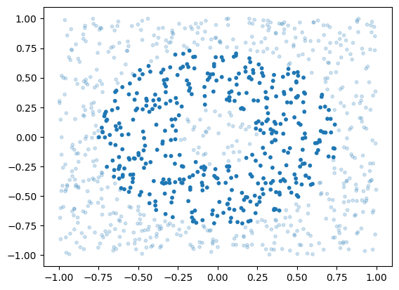
Now let’s generate some data for our quantum circuit to learn from

n_data = 1000
x = random.uniform(random.PRNGKey(0), shape=(n_data, 2), minval=-1, maxval=1)
y = classification_function(x[:, 0], x[:, 1])

plt.scatter(x[:, 0], x[:, 1], alpha=jnp.where(y, 1, 0.2), s=10)

<matplotlib.collections.PathCollection at 0x280c35b50>

Quantum circuit time

We’ll use a variant of data re-uploading Pérez-Salinas et al to encode the input data, alongside some variational parameters within a quantum circuit classifier

n_qubits = 3
depth = 5

c = Circuit(n_qubits)

for layer in range(depth):
    for qi in range(n_qubits):
        c.Rz(0.0, qi)
        c.Ry(0.0, qi)
        c.Rz(0.0, qi)
    if layer < (depth - 1):
        for qi in range(layer, layer + n_qubits - 1, 2):
            c.CZ(qi % n_qubits, (qi + 1) % n_qubits)
        c.add_barrier(range(n_qubits))

render_circuit_jupyter(c)

We can use pytket-qujax to generate our angles-to-statetensor function.

angles_to_st = tk_to_qujax(c)

We’ll parameterise each angle as

\[ \begin{equation} \theta_k = b_k + w_k \, x_k \end{equation} \]

where \(b_k, w_k\) are variational parameters to be learnt and \(x_k = x_0\) if \(k\) even, \(x_k = x_1\) if \(k\) odd for a single bivariate input point \((x_0, x_1)\).

n_angles = 3 * n_qubits * depth
n_params = 2 * n_angles

def param_and_x_to_angles(param, x_single):
    biases = param[:n_angles]
    weights = param[n_angles:]
    weights_times_data = jnp.where(
        jnp.arange(n_angles) % 2 == 0, weights * x_single[0], weights * x_single[1]
    )
    angles = biases + weights_times_data
    return angles

param_and_x_to_st = lambda param, x_single: angles_to_st(
    param_and_x_to_angles(param, x_single)
)

We’ll measure the first qubit only (if its 1 we label donut, if its 0 we label not donut)

def param_and_x_to_probability(param, x_single):
    st = param_and_x_to_st(param, x_single)
    all_probs = jnp.square(jnp.abs(st))
    first_qubit_probs = jnp.sum(all_probs, axis=range(1, n_qubits))
    return first_qubit_probs[1]

For binary classification, the likelihood for our full data set \((x_{1:N}, y_{1:N})\) is

\[ \begin{equation} p(y_{1:N} \mid b, w, x_{1:N}) = \prod_{i=1}^N p(y_i \mid b, w, x_i) = \prod_{i=1}^N (1 - q_{(b,w)}(x_i))^{I[y_i = 0]}q_{(b,w)}(x_i)^{I[y_i = 1]}, \end{equation} \]

where \(q_{(b, w)}(x)\) is the probability the quantum circuit classifies input \(x\) as donut given variational parameter vectors \((b, w)\). This gives log-likelihood

\[ \begin{equation} \log p(y_{1:N} \mid b, w, x_{1:N}) = \sum_{i=1}^N I[y_i = 0] \log(1 - q_{(b,w)}(x_i)) + I[y_i = 1] \log q_{(b,w)}(x_i), \end{equation} \]

which we would like to maximise.

Unfortunately, the log-likelihood cannot be approximated unbiasedly using shots, that is we can approximate \(q_{(b,w)}(x_i)\) unbiasedly but not \(\log(q_{(b,w)}(x_i))\). Note that in qujax simulations we can use the statetensor to calculate this exactly, but it is still good to keep in mind loss functions that can also be used with shots from a quantum device.

Instead we can minimise an expected distance between shots and data

\[ \begin{equation} C(b, w, x, y) = E_{p(y' \mid q_{(b, w)}(x))}[\ell(y', y)] = (1 - q_{(b, w)}(x)) \ell(0, y) + q_{(b, w)}(x)\ell(1, y), \end{equation} \]

where \(y'\) is a shot, \(y\) is a data label and \(\ell\) is some distance between bitstrings - here we simply set \(\ell(0, 0) = \ell(1, 1) = 0\) and \(\ell(0, 1) = \ell(1, 0) = 1\) (which coincides with the Hamming distance for this binary example).

The full batch cost function is

\[ \begin{equation} C(b, w) = \frac1N \sum_{i=1}^N C(b,\, w,\, x_i,\, y_i). \end{equation} \]

Note that to calculate the cost function we need to evaluate the statetensor for every input point \(x_i\). If the dataset becomes too large, we can easily minibatch.

def param_to_cost(param):
    donut_probs = vmap(param_and_x_to_probability, in_axes=(None, 0))(param, x)
    costs = jnp.where(y, 1 - donut_probs, donut_probs)
    return costs.mean()

Ready to descend some gradients?

We’ll just use vanilla gradient descent here

param_to_cost_and_grad = jit(value_and_grad(param_to_cost))

n_iter = 1000
stepsize = 1e-1
param = random.uniform(random.PRNGKey(1), shape=(n_params,), minval=0, maxval=2)
costs = jnp.zeros(n_iter)
for i in range(n_iter):
    cost, grad = param_to_cost_and_grad(param)
    costs = costs.at[i].set(cost)
    param = param - stepsize * grad
    print(i, "Cost: ", cost, end="\r")

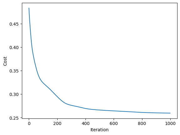
999 Cost:  0.25950647

plt.plot(costs)
plt.xlabel("Iteration")
plt.ylabel("Cost")

Text(0, 0.5, 'Cost')

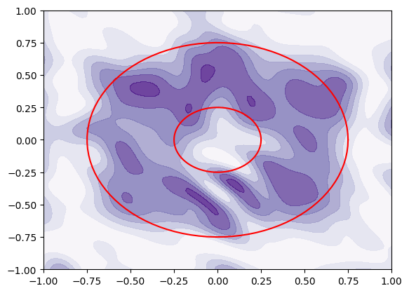
Visualise trained classifier

linsp = jnp.linspace(-1, 1, 100)
Z = vmap(
    lambda a: vmap(lambda b: param_and_x_to_probability(param, jnp.array([a, b])))(
        linsp
    )
)(linsp)

plt.contourf(linsp, linsp, Z, cmap="Purples", alpha=0.8)
circle_linsp = jnp.linspace(0, 2 * jnp.pi, 100)
plt.plot(inner_rad * jnp.cos(circle_linsp), inner_rad * jnp.sin(circle_linsp), c="red")
plt.plot(outer_rad * jnp.cos(circle_linsp), outer_rad * jnp.sin(circle_linsp), c="red")

[<matplotlib.lines.Line2D at 0x284a77910>]

Looks good, it has clearly grasped the donut shape. Sincerest apologies if you are now hungry! 🍩