Training: DisCoCirc
In Section From text to circuit, we saw how to convert entire paragraphs or even documents into quantum circuits using the experimental DisCoCircReader. In lambeq, these circuits can be trained as any other circuit using the standard trainers and models provided by the training module, and we’ll see a concrete example in this section.
For this purpose, we will use a variation of the meaning classification task introduced in [LPM+23], the goal of which was to classify simple sentences as related to IT or food. However, for this example, we will use a dataset of 300 small paragraphs, consisting of 3 sentences each. For example:
Man prepares tasty lunch.
He used to be a good chef.
He likes trying new recipes.
For our training, we will use the PennyLaneModel. We also use a Sim4Ansatz to convert the string diagrams into quantum circuits. When passing these circuits to the PennyLaneModel, they will be automatically converted into PennyLane circuits.
Preparation
We start by specifying some training hyperparameters and importing NumPy and PyTorch.
BATCH_SIZE = 10
EPOCHS = 30
LEARNING_RATE = 0.01
SEED = 42
import random
import numpy as np
import torch
torch.manual_seed(SEED)
random.seed(SEED)
np.random.seed(SEED)
Input data
Let’s read the data and print some example paragraphs.
def read_data(filename):
    labels, sentences = [], []
    with open(filename) as f:
        for line in f:
            t = float(line[0])
            labels.append([t, 1. - t])
            sentences.append(line[1:].strip())
    return labels, sentences
train_labels, train_data = read_data('../examples/datasets/discocirc_mc_train_data.txt')
dev_labels, dev_data = read_data('../examples/datasets/discocirc_mc_dev_data.txt')
test_labels, test_data = read_data('../examples/datasets/discocirc_mc_test_data.txt')
train_data[:5]
['man bakes tasty lunch . he used to be a good shef . he likes mastering new recipes',
 'woman writes efficient program . she has been a great professional . she likes mastering new approaches',
 'girl writes nice software . she is a good coder . she likes mastering novel algorithms',
 'person cooks tasty dinner . he was a modest professional . he likes trying new recipes',
 'man prepares application . he used to be a great coder . he thrives in testing novel algorithms']
Targets are represented as 2-dimensional arrays:
train_labels[:5]
[[1.0, 0.0], [0.0, 1.0], [0.0, 1.0], [1.0, 0.0], [0.0, 1.0]]
Creating and parameterising diagrams
The first step is to convert the paragraphs into string diagrams. For that, we use the experimental DisCoCircReader class. Also, as explained in Section The “sandwich” functor, we need to replace the higher-order DisCoCirc frames into standard boxes by passing sandwich=True to the text2circuit() call to allow conversion to quantum circuits.
from lambeq.experimental.discocirc import DisCoCircReader

reader = DisCoCircReader()

raw_train_diags = [reader.text2circuit(t, sandwich=True) for t in train_data]
raw_dev_diags = [reader.text2circuit(t, sandwich=True) for t in dev_data]
raw_test_diags = [reader.text2circuit(t, sandwich=True) for t in test_data]
We can visualise these diagrams using draw() as usual.
raw_train_diags[0].draw(figsize=(5,10))
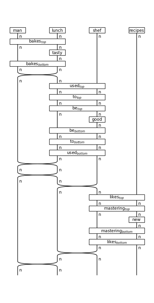
Get a single state for the circuit
For the specific task, we need a means to combine the output wires of the diagram and output a single wire that we will use for the prediction. This is easily done by adding a grammar.Box whose domain is the current diagram output and whose codomain is a single wire which we give the type t for text.
from lambeq import AtomicType
from lambeq.backend.grammar import Box, Ty

# Declare the types we will use
N = AtomicType.NOUN
T = Ty('t')     # 't' for 'text'

# Add fan-in box as last layer for each diagram
def add_fan_in_box(diag):
    fan_in_box = Box(name='fan in',
                     dom=diag.cod,
                     cod=T)
    diag >>= fan_in_box
    return diag

train_diags = [add_fan_in_box(d) for d in raw_train_diags]
dev_diags = [add_fan_in_box(d) for d in raw_dev_diags]
test_diags = [add_fan_in_box(d) for d in raw_test_diags]
train_diags[0].draw(figsize=(6, 10))
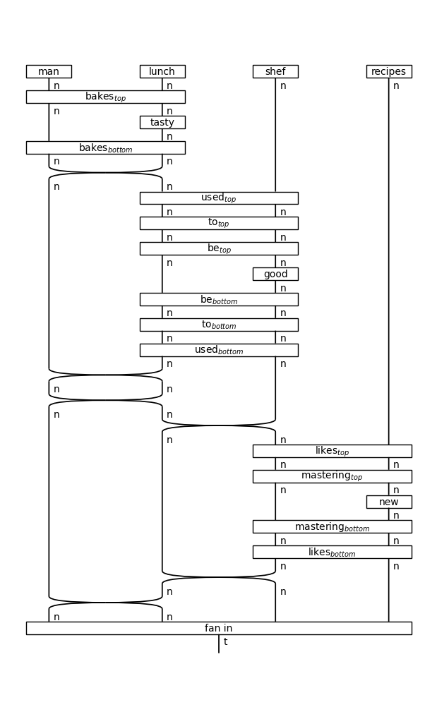
There will be several versions of this “fan in” box, varying only on the number of noun wires in their domain.
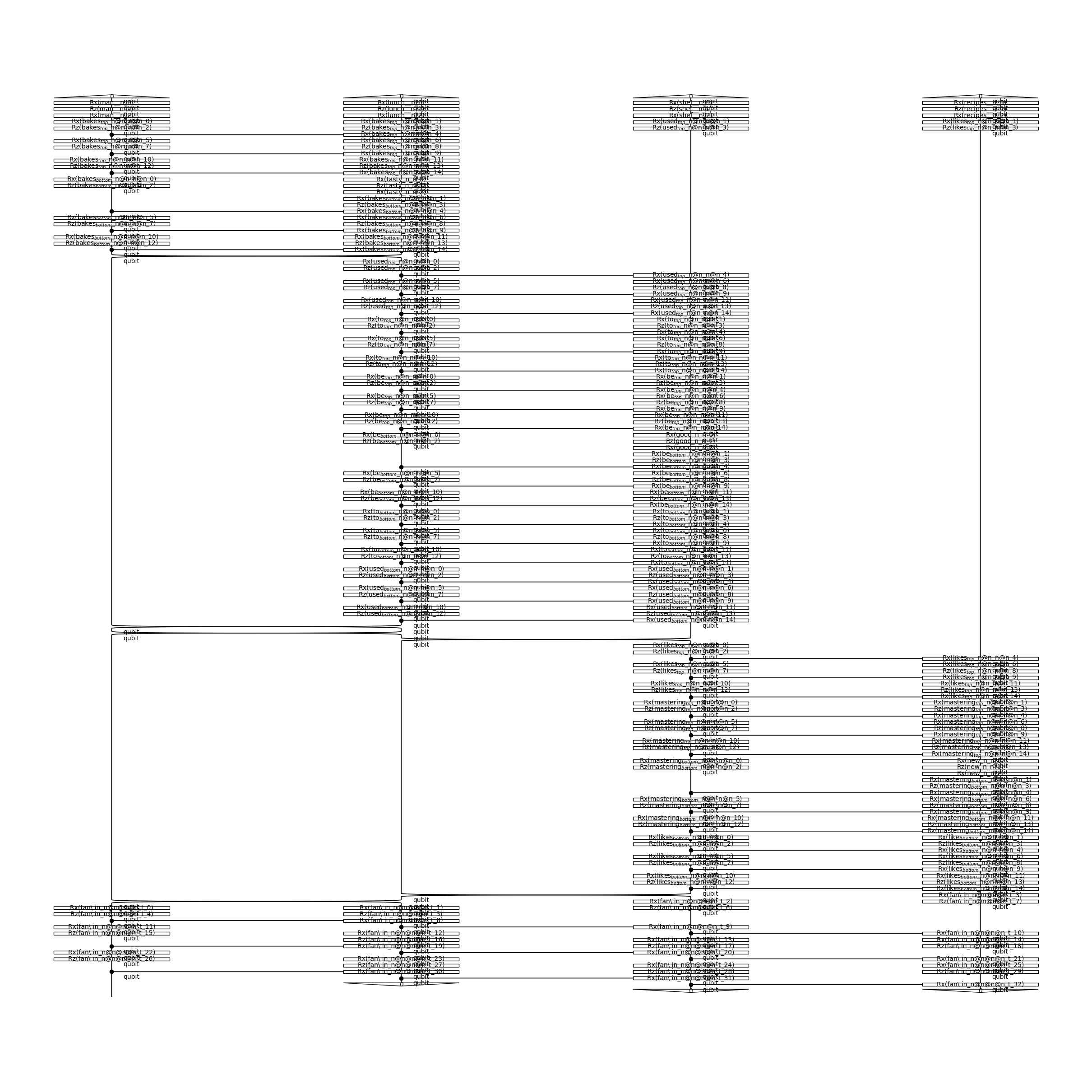
Create circuits
In order to run the experiments on a quantum computer, we apply a quantum ansatz to the string diagrams. As mentioned before, we will use a Sim4Ansatz, where noun wires (n) and text wires (t) are represented by one-qubit systems.
from lambeq import Sim4Ansatz

ansatz = Sim4Ansatz({N: 1, T: 1}, n_layers=3)

train_circs = [ansatz(diag) for diag in train_diags]
dev_circs = [ansatz(diag) for diag in dev_diags]
test_circs = [ansatz(diag) for diag in test_diags]
train_circs[0].draw(figsize=(24, 24))
Training
Instantiate model
We instantiate a PennyLaneModel, by passing all diagrams to the class method from_diagrams(). We also set probabilities=True so that the model outputs probabilities, rather than quantum states, which follows the behaviour of real quantum computers. Furthermore, we set normalize=True so that the output probabilities sum up to one.
from lambeq import PennyLaneModel

all_circs = train_circs + dev_circs + test_circs

# if no backend_config is provided, the default is used
backend_config = {'backend': 'default.qubit'}  # this is the default PennyLane simulator
model = PennyLaneModel.from_diagrams(all_circs,
                                     probabilities=True,
                                     normalize=True,
                                     backend_config=backend_config)
model.initialise_weights()
Running this model on a real quantum computer takes a significant amount of time as the circuits must be sent to the backend and queued, so in this tutorial we will use the default PennyLane simulator, default.qubit.
Create datasets
To facilitate data handling and batching, lambeq provides a native Dataset class. Shuffling is enabled by default, and if not specified, the batch size is set to the length of the dataset.
from lambeq import Dataset

train_dataset = Dataset(train_circs,
                        train_labels,
                        batch_size=BATCH_SIZE)

dev_dataset = Dataset(dev_circs,
                      dev_labels,
                      shuffle=False)
Training can either by done using lambeq’s PytorchTrainer, or by using native PyTorch code. In this tutorial we will be using the first option, which is by far the most straightforward.
Define loss and evaluation metric
We first define our evaluation metrics and loss function, which in this case will be accuracy and binary cross entropy, respectively.
def acc(y_hat, y):
    return (torch.argmax(y_hat, dim=1) ==
            torch.argmax(y, dim=1)).sum().item()/len(y)


def loss(y_hat, y):
    return torch.nn.functional.binary_cross_entropy(
        y_hat, torch.Tensor(y)
    )
Initialise trainer
As PennyLane is compatible with PyTorch autograd, PytorchTrainer can automatically use all of the PyTorch optimizers, such as Adam, to train our model.
from lambeq import PytorchTrainer

trainer = PytorchTrainer(
    model=model,
    loss_function=loss,
    optimizer=torch.optim.Adam,
    learning_rate=LEARNING_RATE,
    epochs=EPOCHS,
    evaluate_functions={'acc': acc},
    evaluate_on_train=True,
    use_tensorboard=False,
    verbose='text',
    seed=SEED)
Train
We can now pass the datasets to the fit() method of the trainer to start the training.
trainer.fit(train_dataset, dev_dataset)
Epoch 1:   train/loss: 0.9695   valid/loss: 1.0455   train/time: 4m15s   valid/time: 1m24s   train/acc: 0.5000   valid/acc: 0.5000
Epoch 2:   train/loss: 1.2423   valid/loss: 0.8468   train/time: 4m18s   valid/time: 1m26s   train/acc: 0.5167   valid/acc: 0.4500
Epoch 3:   train/loss: 1.4184   valid/loss: 0.8690   train/time: 4m19s   valid/time: 1m27s   train/acc: 0.5333   valid/acc: 0.5667
Epoch 4:   train/loss: 0.4773   valid/loss: 1.0767   train/time: 4m20s   valid/time: 1m26s   train/acc: 0.5889   valid/acc: 0.4333
Epoch 5:   train/loss: 0.9689   valid/loss: 0.8239   train/time: 4m23s   valid/time: 1m26s   train/acc: 0.5333   valid/acc: 0.6000
Epoch 6:   train/loss: 0.9354   valid/loss: 0.8176   train/time: 4m25s   valid/time: 1m29s   train/acc: 0.5333   valid/acc: 0.5500
Epoch 7:   train/loss: 1.0967   valid/loss: 0.9583   train/time: 4m27s   valid/time: 1m28s   train/acc: 0.5222   valid/acc: 0.4500
Epoch 8:   train/loss: 0.5902   valid/loss: 0.8774   train/time: 4m28s   valid/time: 1m27s   train/acc: 0.6222   valid/acc: 0.5500
Epoch 9:   train/loss: 0.5998   valid/loss: 0.8630   train/time: 4m43s   valid/time: 1m43s   train/acc: 0.6389   valid/acc: 0.6000
Epoch 10:  train/loss: 0.5799   valid/loss: 0.8210   train/time: 5m11s   valid/time: 1m42s   train/acc: 0.5889   valid/acc: 0.6167
Epoch 11:  train/loss: 0.9772   valid/loss: 1.1537   train/time: 5m11s   valid/time: 1m43s   train/acc: 0.5722   valid/acc: 0.4333
Epoch 12:  train/loss: 0.6276   valid/loss: 0.8586   train/time: 5m14s   valid/time: 1m45s   train/acc: 0.6167   valid/acc: 0.5667
Epoch 13:  train/loss: 1.4431   valid/loss: 1.4355   train/time: 5m17s   valid/time: 1m40s   train/acc: 0.5222   valid/acc: 0.5000
Epoch 14:  train/loss: 0.9701   valid/loss: 0.8888   train/time: 4m29s   valid/time: 1m30s   train/acc: 0.5889   valid/acc: 0.5667
Epoch 15:  train/loss: 0.8250   valid/loss: 0.9828   train/time: 4m34s   valid/time: 1m29s   train/acc: 0.6667   valid/acc: 0.5167
Epoch 16:  train/loss: 1.0572   valid/loss: 0.8387   train/time: 4m28s   valid/time: 1m30s   train/acc: 0.6500   valid/acc: 0.6167
Epoch 17:  train/loss: 0.3985   valid/loss: 0.7681   train/time: 4m31s   valid/time: 1m29s   train/acc: 0.6667   valid/acc: 0.6333
Epoch 18:  train/loss: 0.7628   valid/loss: 0.5444   train/time: 4m31s   valid/time: 1m32s   train/acc: 0.7722   valid/acc: 0.7667
Epoch 19:  train/loss: 0.3056   valid/loss: 0.6176   train/time: 4m32s   valid/time: 1m30s   train/acc: 0.7611   valid/acc: 0.7167
Epoch 20:  train/loss: 0.3587   valid/loss: 0.4453   train/time: 4m32s   valid/time: 1m29s   train/acc: 0.7667   valid/acc: 0.8500
Epoch 21:  train/loss: 0.2189   valid/loss: 0.5145   train/time: 4m32s   valid/time: 1m29s   train/acc: 0.8333   valid/acc: 0.8000
Epoch 22:  train/loss: 0.1592   valid/loss: 0.3655   train/time: 4m31s   valid/time: 1m31s   train/acc: 0.8167   valid/acc: 0.8667
Epoch 23:  train/loss: 0.1945   valid/loss: 0.2800   train/time: 4m32s   valid/time: 1m30s   train/acc: 0.9167   valid/acc: 0.9167
Epoch 24:  train/loss: 0.0599   valid/loss: 0.1828   train/time: 4m33s   valid/time: 1m34s   train/acc: 0.9722   valid/acc: 0.9000
Epoch 25:  train/loss: 0.1717   valid/loss: 0.1657   train/time: 4m35s   valid/time: 1m31s   train/acc: 0.9778   valid/acc: 0.9500
Epoch 26:  train/loss: 0.0121   valid/loss: 0.1378   train/time: 4m37s   valid/time: 1m31s   train/acc: 0.9944   valid/acc: 0.9667
Epoch 27:  train/loss: 0.0367   valid/loss: 0.0807   train/time: 4m40s   valid/time: 1m33s   train/acc: 1.0000   valid/acc: 0.9667
Epoch 28:  train/loss: 0.0038   valid/loss: 0.1031   train/time: 4m36s   valid/time: 1m37s   train/acc: 1.0000   valid/acc: 0.9833
Epoch 29:  train/loss: 0.0083   valid/loss: 0.0597   train/time: 4m38s   valid/time: 1m34s   train/acc: 1.0000   valid/acc: 1.0000
Epoch 30:  train/loss: 0.0065   valid/loss: 0.0595   train/time: 4m34s   valid/time: 1m32s   train/acc: 1.0000   valid/acc: 1.0000

Training completed!
train/time: 2h17m57s   train/time_per_epoch: 4m36s   train/time_per_step: 15.33s   valid/time: 45m57s   valid/time_per_eval: 1m32s
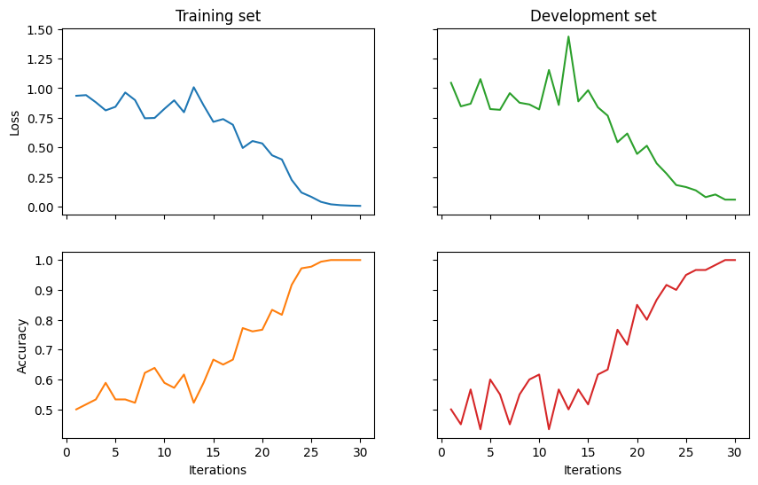
Results
Finally, we visualise the results and evaluate the model on the test data.
import matplotlib.pyplot as plt


fig, ((ax_tl, ax_tr), (ax_bl, ax_br)) = plt.subplots(2, 2,
                                                     sharex=True,
                                                     sharey='row',
                                                     figsize=(10, 6))
ax_tl.set_title('Training set')
ax_tr.set_title('Development set')
ax_bl.set_xlabel('Iterations')
ax_br.set_xlabel('Iterations')
ax_bl.set_ylabel('Accuracy')
ax_tl.set_ylabel('Loss')

colours = iter(plt.rcParams['axes.prop_cycle'].by_key()['color'])
range_ = np.arange(1, trainer.epochs+1)
ax_tl.plot(range_, trainer.train_epoch_costs, color=next(colours))
ax_bl.plot(range_, trainer.train_eval_results['acc'], color=next(colours))
ax_tr.plot(range_, trainer.val_costs, color=next(colours))
ax_br.plot(range_, trainer.val_eval_results['acc'], color=next(colours))

# print test accuracy
pred = model(test_circs)
labels = torch.tensor(test_labels)

print('Final test accuracy: {}'.format(acc(pred, labels)))
Final test accuracy: 0.9666666666666667
See also: