H-Series Emulators

An emulator can be used to get an idea of what a quantum device will output for a given quantum circuit. This enables circuit debugging and optimization before running on a physical machine. Emulators differ from simulators in that they model the physical and noise model of the device whereas simulators may model noise parameters, but not physical parameters.

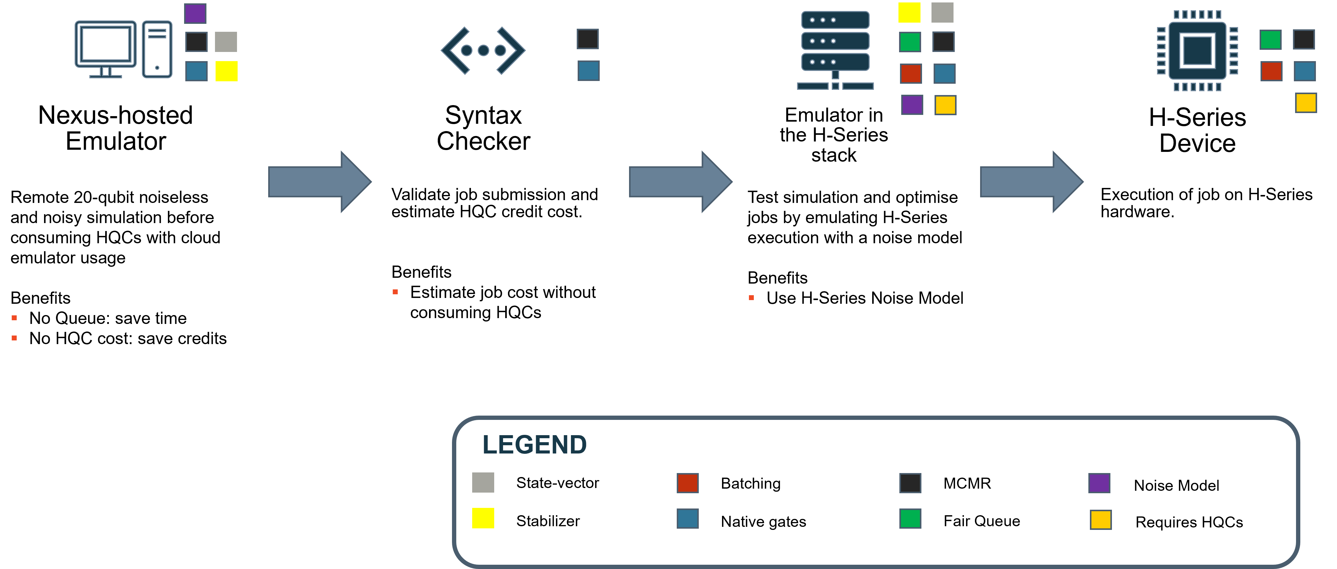
The Quantinuum emulators run on a physical noise model of the Quantinuum H-Series devices. There are various noise/error parameters modeled. For detailed information on the noise model, see the emulator data sheets on the System Model H1 or System Model H2 pages. There are cloud emulators and local emulators available.

• State vector Emulator: The default mode of all emulators. The emulator will compute the state vector of the circuit and estimate the measurement distribution from that state vector. (option: state-vector)

• Stabilizer Emulator: Use of the emulator for circuits involving only Clifford operations. This is only available on cloud emulators (option: stabilizer)

• Noiseless Emulation: Disable the noise model for state vector and stabilizer emulators. Only shot noise is present in the emulation result. The pytket-pecos package enables noiseless (state-vector) emulation locally. The Cloud emulators enable noiseless emulation by setting error-model to False.

• Noise Model Customization: Experiment with the noise parameters in the emulator. There is no guarantee that results achieved changing these parameters will represent outputs from the actual quantum computer represented. This is only available for the cloud emulators.

Emulator Availability and Usage

All H-Series devices have cloud emulators (suffix E) and local emulators (suffix LE).

Users can access cloud emulators with their Quantinuum credentials over the cloud via the Fair Queue. These emulators are hosted on Quantinuum’s infrastructure, consume HQCs upon usage, are available 24/7, and replicate H-Series device and noise characteristics unless the user utilizes the noise model options. Cloud emulators are accessible via pytket-quantinuum.

User can also access local emulators. Local emulators do not consume HQCs and only provide noiseless emulation modeling physical characteristics like transport, but not noise. Only state-vector simulation is available for local emulators. The user does not need to submit jobs to a queue. Local emulators are accessible via pytket-pecos and pytket-quantinuum.

For smaller noiseless emulations involving less than 16 qubits, it is recommended to use the local emulators. For larger emulations, or emulations using a noise model, cloud emulators is recommended.

Targets:

• H1-1E

• H1-1LE

• H2-1E

• H2-1LE

All emulators provide the following features:

• Usage of arbitrary-angle 2-qubit gates as well as other native H-Series gates

• All-to-all connectivity

• Mid-circuit measurements and reset (MCMR) and qubit reuse

• Identical number of qubits to the corresponding device (i.e. H2-1E and H2-1LE both have 32 qubits maximum) for state-vector simulation.

Cloud emulators provide the following features:

• Job Batching (run all jobs by a user in succession)

• A noise model replicating device noise characteristics

• state-vector and stabilizer simulators. State-vector simulators have up to 32 qubits. Stabilizer simulator has up to 1000 qubits.

Cloud emulators can only be accessed via the Fair Queue. Queue time is dependent on HQC accumulation and user- and group-priorities within their organization. Emulator run-time is dependent on the number of qubits and number of operations in the job. Noisy emulations are slower than noiseless emulations.

Jobs submitted to the cloud emulator with a high shot count are automatically chunked into multiple partitions with fewer shots. This enables an incremental distribution of emulator resources.

Basic Usage

In the cell below, a QuantinuumBackend is constructed with the device_name argument specified as the H1-1 emulator (H1-1E). The QuantinuumBackend instance will be used to:

• Compile the circuit to satisfy the gate set predicate for the emulator using the instance get_compiled_circuit method.

• Cost the circuit to identify HQC consumption for emulation using the instance cost method.

• Submit the circuit for emulation via process_circuit.

• Check job status for the submitted circuit with circuit_status.

• Retrieve job result after emulation with get_result.

This workflow is identical for both Quantum Processing Unit (QPU) usage and emulator usage.

This workflow is the default (and simplest) for the H-Series emulators. In most cases, we recommend users use this workflow since it will mimic device performance.

from pytket.extensions.quantinuum import QuantinuumBackend

backend = QuantinuumBackend("H1-1E")
backend.login()

Enter your Quantinuum email: irfan.khan@quantinuum.com
Enter your Quantinuum password: ········

All devices accessible to the user are visible through the QuantinuumBackend.available_devices method.

backend.available_devices()[1]

BackendInfo(name='QuantinuumBackend', device_name='H1-1E', version='0.30.0', architecture=<tket::FullyConnected, nodes=20>, gate_set={<OpType.Reset: 65>, <OpType.Rz: 36>, <OpType.PhasedX: 68>, <OpType.ZZMax: 70>, <OpType.Barrier: 8>, <OpType.ClassicalExpBox: 104>, <OpType.ZZPhase: 73>, <OpType.TK2: 41>, <OpType.WASM: 14>, <OpType.SetBits: 15>, <OpType.CopyBits: 16>, <OpType.RangePredicate: 17>, <OpType.ExplicitPredicate: 18>, <OpType.ExplicitModifier: 19>, <OpType.MultiBit: 20>, <OpType.Measure: 63>}, n_cl_reg=120, supports_fast_feedforward=True, supports_reset=True, supports_midcircuit_measurement=True, all_node_gate_errors=None, all_edge_gate_errors=None, all_readout_errors=None, averaged_node_gate_errors=None, averaged_edge_gate_errors=None, averaged_readout_errors=None, misc={'wasm': True, 'batching': True, 'max_n_shots': 10000, 'system_type': 'emulator', 'cl_reg_width': 32})

The 4-qubit circuit below contains the following features:

• Native arbitrary-angle 2-qubit gate (OpType.ZZPhase)

• Native arbitrary-angle 1-qubit gate (OpType.PhasedX)

• MCMR (mid-circuit measurement with reset)

• Classically-controlled OpType.X operation

from pytket.circuit import Circuit
from pytket.circuit.display import render_circuit_jupyter

circuit = Circuit(4, 1)
for i, j in zip(circuit.qubits[:-1], circuit.qubits[1:]):
    circuit.ZZPhase(0.1, i, j)

# Add MCMR
circuit.Measure(circuit.qubits[-1], circuit.bits[0])
circuit.Reset(circuit.qubits[-1])
circuit.X(circuit.qubits[-1], condition=circuit.bits[0])

for i, j in zip(circuit.qubits[:-1], circuit.qubits[1:]):
    circuit.ZZPhase(0.1, i, j)
for i in circuit.qubits:
    circuit.PhasedX(0.06, -0.09, i)

## Add Final Measurement
circuit.measure_all()

render_circuit_jupyter(circuit)

Compiling the circuit with QuantinuumBackend, replaces the classically-controlled OpType.X operation with an OpType.Phase node and a classically-controlled Optype.PhasedX.

compiled_circuit = backend.get_compiled_circuit(circuit, optimisation_level=2)

render_circuit_jupyter(compiled_circuit)

The compiled circuit can be submitted to the H1-1SC to estimate HQC consumption for emulation via the cost function.

hqc_cost = backend.cost(compiled_circuit, n_shots=100, syntax_checker="H1-1SC")
print(hqc_cost)

7.46

process_circuit is used to submit the compiled circuit for emulation.

handle = backend.process_circuit(compiled_circuit, n_shots=100)

The ResultHandle object, a reference to the job submitted to the H-Series emulator, is saved to disk with json.

import json

with open("result_handle.json", "w") as json_io:
    json.dump([str(handle)], json_io)

The ResultHandle data is loaded from disk and used to instantiate a ResultHandle object.

from pytket.backends.resulthandle import ResultHandle

with open("result_handle.json", "r") as json_io:
    result_handle_str_list = json.load(json_io)
    handle = ResultHandle.from_str(result_handle_str_list[0])

The ResultHandle object is used to query the status of the job submitted to the H-Series emulator.

job_status = backend.circuit_status(handle)
print(job_status)

CircuitStatus(status=<StatusEnum.QUEUED: 'Circuit is queued.'>, message='{"name": "job", "submit-date": "2024-04-02T15:12:46.676648", "result-date": null, "queue-position": null, "cost": "7.46", "error": null}', error_detail=None, completed_time=None, queued_time=None, submitted_time=None, running_time=None, cancelled_time=None, error_time=None, queue_position=None)

get_result can be used to retrieve the job result after H-Series emulation is complete.

result = backend.get_result(handle)

State vector and Stabilizer Emulator

The following options can only be used when using the cloud H-Series emulators (ending with E and not LE).

There are two types of simulation methods, state-vector and stabilizer. These can be specified during construction of QuantinuumBackend via the simulator keyword argument. The default value is state-vector.

If the quantum operations are all Clifford gates, it is faster to use the stabilizer emulator. The stabilizer emulator is requested in the setup of the QuantinuumBackend with the simulator input option. This option can only be used with cloud H-Series emulators.

machine = "H1-1E"
stabilizer_backend = QuantinuumBackend(device_name=machine, simulator="stabilizer")

print(machine, "status:", stabilizer_backend.device_state(device_name=machine))
print("Simulation type:", stabilizer_backend.simulator_type)

H1-1E status: online
Simulation type: stabilizer

backend.get_compiled_circuit(Circuit(2).CX(0, 1), optimisation_level=2)

[PhasedX(0.5, 0.5) q[1]; ZZPhase(0.5) q[0], q[1]; Rz(0.5) q[0]; PhasedX(0.5, 0) q[1]; Rz(1.5) q[1]; ]

Noiseless Emulation

Enabling and Disabling the Error Model with the Cloud Emulators

Quantinuum emulators may be run with or without the physical device’s noise model. The default is the emulator runs with the physical noise model turned on. The physical noise model can be turned off by setting noisy_simulation=False. Noiseless simulation can be used with both state-vector and stabilizer emulator.

from pytket.circuit import Circuit

circuit = Circuit(4)
for _ in range(2):
    for i in circuit.qubits:
        circuit.PhasedX(-0.1, -0.2, i)
circuit.measure_all()

compiled_circuit = backend.get_compiled_circuit(circuit)

The process_circuit method can be used with the keyword argument noisy_simulation.

n_shots = 100
no_error_model_handle = backend.process_circuit(
    compiled_circuit, n_shots=n_shots, noisy_simulation=False
)

An alternative setup is to specify the Quantinuum API option, error-model as False, during construction of QuantinuumBackend.

backend_noiseless = QuantinuumBackend(
    device_name="H1-1E", options={"error-model": "False"}
)

Local Emulation using pytket-pecos

To use the local emulators, pytket-quantinuum needs to be installed using the extra install argument pecos. All local emulators are state-vector simulators.

• Installation command: pip install pytket-quantinuum[pecos]

This provides local emulator targets. Each device has a corresponding local emulator, with the suffix LE added to the device name.

• H1-1LE

• H2-1LE

After installation, the end user can verify the local emulators are usable with the method have_pecos with boolean output.

from pytket.extensions.quantinuum import have_pecos

have_pecos()

True

The methods, process_circuit and process_circuits, provide a keyword argument, mulithreading, to accelerate local emulation. This can be toggled True to use.

qntm_backend_le = QuantinuumBackend(device_name="H1-1LE")

handle = qntm_backend_le.process_circuit(
    compiled_circuit, n_shots=100, multithreading=True
)

Noise Model Customization

The emulator runs with default error parameters that represent a noise environment similar to the physical devices. For detailed information on the noise model, see the product data sheet for the device you want to emulate on the System Model H1 or System Model H2 page.

The error-params option can be used to customize the noise model. This can be supplied either to:

• the QuantinuumBackend constructor with arguments error-model or error-params within the options keyword argument

• the process_circuit or process_circuits method with the keyword argument options

Within the options argument, the two options below are provided for controlling the noise model:

• error-model: A boolean to specify if the error model should be enabled (True) or disabled (False). By default the error model is enabled.

• error-params: If the error model is enabled, a nested dictionary is provided containing the error model parameters to tweak.

In this section, examples are given for experimenting with the noise and error parameters of the emulators. These are advanced options and not recommended to start with when doing initial experiments. As mentioned above, there is no guarantee that results achieved changing these parameters will represent outputs from the actual quantum computer represented.

Note: All the noise parameters are used together any time a simulation is run. If only some of the parameters are specified, the rest of the parameters are used at their default settings. The parameters to override are specified with the options parameter.

The example below specifies the options with the QuantinuumBackend constructor.

options = {"error-model": True, "error-params": {"quadratic_dephasing_rate": 0.1}}

qntm_backend_custom = QuantinuumBackend(device_name="H2-1E", options=options)

The example below instead utilizes the error model options within the process_circuit function.

backend = QuantinuumBackend(device_name="H1-1E", options={"error-params": {"p1": 1e-5}})

handle = backend.process_circuit(
    compiled_circuit, n_shots=10, options={"error-params": {"p2": 1e-4}}
)

Physical Noise

See the product data sheet for the device you want to emulate for information on these parameters.

backend = QuantinuumBackend(
    device_name="H1-1E",
    options={
        "error-params": {
            "p1": 4e-5,
            "p2": 3e-3,
            "p_meas": 3e-3,
            "p_init": 4e-5,
            "p_crosstalk_meas": 1e-5,
            "p_crosstalk_init": 3e-5,
            "p1_emission_ratio": 0.15,
            "p2_emission_ratio": 0.3,
        }
    },
)

Dephasing Noise

The noise model includes a memory error for which Pauli-\(Z\) is applied. This is often called “dephasing” or “memory” noise. There are two relationships between the probability of dephasing error and the duration for which qubits are idling or transporting in the trap:

1. the probability is quadratically dependent on the duration

2. the probability is linearly dependent on the duration

For both the state-vector and stabilizer simulations, linear dephasing is also modeled with Pauli-\(Z\) applied with a probability equal to rate, \(r\), multiplied by duration, \(d\).

For state-vector simulations, the quadratic noise is modeled in the emulator by default as coherent noise. For this coherent quadratic dephasing noise, the \(Rz\) gate is applied with an angle proportional to frequency, \(f\), multiplied by duration, \(d\). The probability of the \(Rz\) gate applying a Pauli-\(Z\) operation on a plus state, \(| + \rangle\), is \(\sin( fd/2 )^2\), which is why we call this a form of quadratic dephasing.

For the stabilizer simulator, by default this quadratic noise is modeled incoherent by applying Pauli-\(Z\) with probability \(\sin{(fd)}^2\) to model more closely the quadratic dependency with frequency and time as seen in the coherent model. Note, stabilizer simulations can only simulate Clifford and measurement-like gates, so the \(Rz\) gate cannot be applied directly.

See the product data sheet for the device you want to emulate for information on these parameters.

backend = QuantinuumBackend(
    device_name="H1-1E",
    options={
        "error-params": {
            "quadratic_dephasing_rate": 0.2,
            "linear_dephasing_rate": 0.3,
            "coherent_to_incoherent_factor": 2.0,
            "coherent_dephasing": False,  # False => run the incoherent noise model
            "transport_dephasing": False,  # False => turn off transport dephasing error
            "idle_dephasing": False,  # False => turn off idle dephasing error
        },
    },
)

Arbitrary Angle Noise Scaling

The System Model H1 systems have a native arbitrary-angle \(ZZ\) gate, \(RZZ(\theta)\). For implementation of this gate in the System Model H1 emulator, certain parameters relate to the strength of the asymmetric depolarizing noise. These parameters depend on the angle \(\theta\). This is normalized so that \(\theta=\pi/2\) gives the 2-qubit fault probability (p2). The parameters for asymmetric depolarizing noise are fit parameters that fit the noise estimated as the angle, \(\theta\), changes per this equation:

The parameters for asymmetric depolarizing noise are fit parameters that fit the noise estimated as the angle, \(\theta\), changes per this equation:

\begin{align} (przz_a (|\theta|/\pi)^{przz_{power}} + przz_b) p2; \quad &\theta &< 0 \

(przz_c (|\theta|/\pi)^{przz_{power}} + przz_d) p2; \quad &\theta &> 0 \

0.5 (przz_b + przz_d); \quad &\theta &= 0 \end{align}

See the product data sheet for the device you want to emulate for information on these parameters.

backend = QuantinuumBackend(
    device_name="H1-1E",
    options={
        "error-params": {
            "przz_a": 1.09,
            "przz_b": 0.035,
            "przz_c": 1.09,
            "przz_d": 0.035,
            "przz_power": 1 / 2,
        },
    },
)

Scaling Factors

A scaling factor can be applied that multiplies all the default or supplied error parameters by the scaling rate. In this case, a 1 does not change the error rates while 0 makes all the errors have a probability of 0.

All the error rates can be scaled linearly using the scale parameter.

backend = QuantinuumBackend(
    device_name="H1-1E",
    options={
        "error-params": {
            "scale": 0.1,
        },
    },
)

See the product data sheet for the device you want to emulate for information on these parameters.

backend = QuantinuumBackend(
    device_name="H1-1E",
    options={
        "error-params": {
            "p1_scale": 0.1,
            "p2_scale": 0.1,
            "meas_scale": 0.1,
            "init_scale": 0.1,
            "memory_scale": 0.1,
            "emission_scale": 0.1,
            "crosstalk_scale": 0.1,
            "leakage_scale": 0.1,
        },
    },
)

Use Case: Noise Model Analysis

The noise model can be configured on the state-vector simulator in order to assess performance improvements for a particular use case as certain hardware noise parameters (i.e. the 2-qubit gate fidelity improves).

This use case looks at the Jensen-Shannon divergence (JSD) as the p2 noise model value is modified. JSD is a measure of result quality, 0 is the maximal quality and 1 is the worst. A random circuit is submitted to the emulator for 5 different values of p2. The JSD can be computed once results are available from the noisy emulation. Emulation results are compared to results from an ideal case, and this is a benchmark for similarity between the two measurement distributions.

The code cell below generates 5 p2 values between 0 and 0.1.

import numpy as np

p2_list = np.linspace(0, 0.1, num=5, endpoint=True)

The code below generates a 10-qubit circuit with 10 repeating sub-blocks. Each sub-block contains OpType.PhasedX and OpType.ZZPhase operations.

from pytket.circuit import Circuit

circuit = Circuit(10)

for i in range(10):
    for j, qubit in enumerate(circuit.qubits):
        a0 = j * 0.05**i
        a1 = j * 0.1**i
        circuit.PhasedX(a0, a1, qubit)

    for j, (q0, q1) in enumerate(zip(circuit.qubits[:-1], circuit.qubits[1:])):
        angle = 0.1**i
        circuit.ZZPhase(0.1, q0, q1)

circuit.measure_all()

[PhasedX(0, 0) q[0]; PhasedX(1, 1) q[1]; PhasedX(2, 0) q[2]; PhasedX(3, 1) q[3]; PhasedX(0, 0) q[4]; PhasedX(1, 1) q[5]; PhasedX(2, 0) q[6]; PhasedX(3, 1) q[7]; PhasedX(0, 0) q[8]; PhasedX(1, 1) q[9]; ZZPhase(0.1) q[0], q[1]; PhasedX(0, 0) q[0]; ZZPhase(0.1) q[1], q[2]; PhasedX(0.05, 0.1) q[1]; ZZPhase(0.1) q[2], q[3]; ZZPhase(0.1) q[0], q[1]; PhasedX(0.1, 0.2) q[2]; ZZPhase(0.1) q[3], q[4]; PhasedX(0, 0) q[0]; ZZPhase(0.1) q[1], q[2]; PhasedX(0.15, 0.3) q[3]; ZZPhase(0.1) q[4], q[5]; PhasedX(0.0025, 0.01) q[1]; ZZPhase(0.1) q[2], q[3]; PhasedX(0.2, 0.4) q[4]; ZZPhase(0.1) q[5], q[6]; ZZPhase(0.1) q[0], q[1]; PhasedX(0.005, 0.02) q[2]; ZZPhase(0.1) q[3], q[4]; PhasedX(0.25, 0.5) q[5]; ZZPhase(0.1) q[6], q[7]; PhasedX(0, 0) q[0]; ZZPhase(0.1) q[1], q[2]; PhasedX(0.0075, 0.03) q[3]; ZZPhase(0.1) q[4], q[5]; PhasedX(0.3, 0.6) q[6]; ZZPhase(0.1) q[7], q[8]; PhasedX(0.000125, 0.001) q[1]; ZZPhase(0.1) q[2], q[3]; PhasedX(0.01, 0.04) q[4]; ZZPhase(0.1) q[5], q[6]; PhasedX(0.35, 0.7) q[7]; ZZPhase(0.1) q[8], q[9]; ZZPhase(0.1) q[0], q[1]; PhasedX(0.00025, 0.002) q[2]; ZZPhase(0.1) q[3], q[4]; PhasedX(0.0125, 0.05) q[5]; ZZPhase(0.1) q[6], q[7]; PhasedX(0.4, 0.8) q[8]; PhasedX(0.45, 0.9) q[9]; PhasedX(0, 0) q[0]; ZZPhase(0.1) q[1], q[2]; PhasedX(0.000375, 0.003) q[3]; ZZPhase(0.1) q[4], q[5]; PhasedX(0.015, 0.06) q[6]; ZZPhase(0.1) q[7], q[8]; PhasedX(6.25e-06, 0.0001) q[1]; ZZPhase(0.1) q[2], q[3]; PhasedX(0.0005, 0.004) q[4]; ZZPhase(0.1) q[5], q[6]; PhasedX(0.0175, 0.07) q[7]; ZZPhase(0.1) q[8], q[9]; ZZPhase(0.1) q[0], q[1]; PhasedX(1.25e-05, 0.0002) q[2]; ZZPhase(0.1) q[3], q[4]; PhasedX(0.000625, 0.005) q[5]; ZZPhase(0.1) q[6], q[7]; PhasedX(0.02, 0.08) q[8]; PhasedX(0.0225, 0.09) q[9]; PhasedX(0, 0) q[0]; ZZPhase(0.1) q[1], q[2]; PhasedX(1.875e-05, 0.0003) q[3]; ZZPhase(0.1) q[4], q[5]; PhasedX(0.00075, 0.006) q[6]; ZZPhase(0.1) q[7], q[8]; PhasedX(3.125e-07, 1e-05) q[1]; ZZPhase(0.1) q[2], q[3]; PhasedX(2.5e-05, 0.0004) q[4]; ZZPhase(0.1) q[5], q[6]; PhasedX(0.000875, 0.007) q[7]; ZZPhase(0.1) q[8], q[9]; ZZPhase(0.1) q[0], q[1]; PhasedX(6.25e-07, 2e-05) q[2]; ZZPhase(0.1) q[3], q[4]; PhasedX(3.125e-05, 0.0005) q[5]; ZZPhase(0.1) q[6], q[7]; PhasedX(0.001, 0.008) q[8]; PhasedX(0.001125, 0.009) q[9]; PhasedX(0, 0) q[0]; ZZPhase(0.1) q[1], q[2]; PhasedX(9.375e-07, 3e-05) q[3]; ZZPhase(0.1) q[4], q[5]; PhasedX(3.75e-05, 0.0006) q[6]; ZZPhase(0.1) q[7], q[8]; PhasedX(1.5625e-08, 1e-06) q[1]; ZZPhase(0.1) q[2], q[3]; PhasedX(1.25e-06, 4e-05) q[4]; ZZPhase(0.1) q[5], q[6]; PhasedX(4.375e-05, 0.0007) q[7]; ZZPhase(0.1) q[8], q[9]; ZZPhase(0.1) q[0], q[1]; PhasedX(3.125e-08, 2e-06) q[2]; ZZPhase(0.1) q[3], q[4]; PhasedX(1.5625e-06, 5e-05) q[5]; ZZPhase(0.1) q[6], q[7]; PhasedX(5e-05, 0.0008) q[8]; PhasedX(5.625e-05, 0.0009) q[9]; PhasedX(0, 0) q[0]; ZZPhase(0.1) q[1], q[2]; PhasedX(4.6875e-08, 3e-06) q[3]; ZZPhase(0.1) q[4], q[5]; PhasedX(1.875e-06, 6e-05) q[6]; ZZPhase(0.1) q[7], q[8]; PhasedX(7.8125e-10, 1e-07) q[1]; ZZPhase(0.1) q[2], q[3]; PhasedX(6.25e-08, 4e-06) q[4]; ZZPhase(0.1) q[5], q[6]; PhasedX(2.1875e-06, 7e-05) q[7]; ZZPhase(0.1) q[8], q[9]; ZZPhase(0.1) q[0], q[1]; PhasedX(1.5625e-09, 2e-07) q[2]; ZZPhase(0.1) q[3], q[4]; PhasedX(7.8125e-08, 5e-06) q[5]; ZZPhase(0.1) q[6], q[7]; PhasedX(2.5e-06, 8e-05) q[8]; PhasedX(2.8125e-06, 9e-05) q[9]; PhasedX(0, 0) q[0]; ZZPhase(0.1) q[1], q[2]; PhasedX(2.34375e-09, 3e-07) q[3]; ZZPhase(0.1) q[4], q[5]; PhasedX(9.375e-08, 6e-06) q[6]; ZZPhase(0.1) q[7], q[8]; PhasedX(3.90625e-11, 1e-08) q[1]; ZZPhase(0.1) q[2], q[3]; PhasedX(3.125e-09, 4e-07) q[4]; ZZPhase(0.1) q[5], q[6]; PhasedX(1.09375e-07, 7e-06) q[7]; ZZPhase(0.1) q[8], q[9]; ZZPhase(0.1) q[0], q[1]; PhasedX(7.8125e-11, 2e-08) q[2]; ZZPhase(0.1) q[3], q[4]; PhasedX(3.90625e-09, 5e-07) q[5]; ZZPhase(0.1) q[6], q[7]; PhasedX(1.25e-07, 8e-06) q[8]; PhasedX(1.40625e-07, 9e-06) q[9]; PhasedX(0, 0) q[0]; ZZPhase(0.1) q[1], q[2]; PhasedX(1.17188e-10, 3e-08) q[3]; ZZPhase(0.1) q[4], q[5]; PhasedX(4.6875e-09, 6e-07) q[6]; ZZPhase(0.1) q[7], q[8]; PhasedX(0, 1e-09) q[1]; ZZPhase(0.1) q[2], q[3]; PhasedX(1.5625e-10, 4e-08) q[4]; ZZPhase(0.1) q[5], q[6]; PhasedX(5.46875e-09, 7e-07) q[7]; ZZPhase(0.1) q[8], q[9]; ZZPhase(0.1) q[0], q[1]; PhasedX(0, 2e-09) q[2]; ZZPhase(0.1) q[3], q[4]; PhasedX(1.95313e-10, 5e-08) q[5]; ZZPhase(0.1) q[6], q[7]; PhasedX(6.25e-09, 8e-07) q[8]; PhasedX(7.03125e-09, 9e-07) q[9]; Measure q[0] --> c[0]; ZZPhase(0.1) q[1], q[2]; PhasedX(0, 3e-09) q[3]; ZZPhase(0.1) q[4], q[5]; PhasedX(2.34375e-10, 6e-08) q[6]; ZZPhase(0.1) q[7], q[8]; Measure q[1] --> c[1]; ZZPhase(0.1) q[2], q[3]; PhasedX(0, 4e-09) q[4]; ZZPhase(0.1) q[5], q[6]; PhasedX(2.73438e-10, 7e-08) q[7]; ZZPhase(0.1) q[8], q[9]; Measure q[2] --> c[2]; ZZPhase(0.1) q[3], q[4]; PhasedX(0, 5e-09) q[5]; ZZPhase(0.1) q[6], q[7]; PhasedX(3.125e-10, 8e-08) q[8]; PhasedX(3.51563e-10, 9e-08) q[9]; Measure q[3] --> c[3]; ZZPhase(0.1) q[4], q[5]; PhasedX(1.17188e-11, 6e-09) q[6]; ZZPhase(0.1) q[7], q[8]; Measure q[4] --> c[4]; ZZPhase(0.1) q[5], q[6]; PhasedX(1.36719e-11, 7e-09) q[7]; ZZPhase(0.1) q[8], q[9]; Measure q[5] --> c[5]; ZZPhase(0.1) q[6], q[7]; PhasedX(1.5625e-11, 8e-09) q[8]; PhasedX(1.75781e-11, 9e-09) q[9]; Measure q[6] --> c[6]; ZZPhase(0.1) q[7], q[8]; Measure q[7] --> c[7]; ZZPhase(0.1) q[8], q[9]; Measure q[8] --> c[8]; Measure q[9] --> c[9]; ]

The local (noiseless) emulator, H1-1LE, is used to obtain a distribution of measurement outcomes in the ideal case.

backend_noiseless = QuantinuumBackend(device_name="H1-1LE")

result_ideal = backend_noiseless.run_circuit(circuit, n_shots=100)

print(result_ideal.get_distribution())

{(0, 0, 0, 1, 0, 1, 0, 1, 0, 1): 0.01, (0, 1, 0, 0, 0, 0, 0, 1, 1, 1): 0.01, (0, 1, 0, 0, 0, 1, 0, 0, 0, 0): 0.01, (0, 1, 0, 0, 0, 1, 0, 1, 0, 0): 0.01, (0, 1, 0, 0, 0, 1, 0, 1, 0, 1): 0.01, (0, 1, 0, 0, 0, 1, 0, 1, 1, 0): 0.01, (0, 1, 0, 0, 1, 1, 0, 1, 0, 0): 0.02, (0, 1, 0, 0, 1, 1, 0, 1, 1, 0): 0.01, (0, 1, 0, 0, 1, 1, 1, 1, 0, 0): 0.01, (0, 1, 0, 1, 0, 0, 0, 0, 0, 1): 0.01, (0, 1, 0, 1, 0, 0, 0, 0, 1, 0): 0.01, (0, 1, 0, 1, 0, 0, 0, 1, 0, 0): 0.01, (0, 1, 0, 1, 0, 0, 0, 1, 0, 1): 0.03, (0, 1, 0, 1, 0, 0, 0, 1, 1, 0): 0.02, (0, 1, 0, 1, 0, 0, 0, 1, 1, 1): 0.01, (0, 1, 0, 1, 0, 0, 1, 0, 0, 0): 0.01, (0, 1, 0, 1, 0, 0, 1, 1, 0, 1): 0.02, (0, 1, 0, 1, 0, 0, 1, 1, 1, 1): 0.01, (0, 1, 0, 1, 0, 1, 0, 0, 0, 0): 0.04, (0, 1, 0, 1, 0, 1, 0, 0, 0, 1): 0.05, (0, 1, 0, 1, 0, 1, 0, 0, 1, 0): 0.02, (0, 1, 0, 1, 0, 1, 0, 0, 1, 1): 0.01, (0, 1, 0, 1, 0, 1, 0, 1, 0, 0): 0.09, (0, 1, 0, 1, 0, 1, 0, 1, 0, 1): 0.22, (0, 1, 0, 1, 0, 1, 0, 1, 1, 0): 0.06, (0, 1, 0, 1, 0, 1, 0, 1, 1, 1): 0.05, (0, 1, 0, 1, 0, 1, 1, 0, 0, 0): 0.03, (0, 1, 0, 1, 0, 1, 1, 0, 0, 1): 0.01, (0, 1, 0, 1, 0, 1, 1, 0, 1, 0): 0.01, (0, 1, 0, 1, 0, 1, 1, 0, 1, 1): 0.01, (0, 1, 0, 1, 0, 1, 1, 1, 0, 0): 0.04, (0, 1, 0, 1, 0, 1, 1, 1, 0, 1): 0.06, (0, 1, 0, 1, 0, 1, 1, 1, 1, 0): 0.01, (0, 1, 0, 1, 0, 1, 1, 1, 1, 1): 0.01, (0, 1, 0, 1, 1, 1, 0, 1, 1, 1): 0.01, (0, 1, 0, 1, 1, 1, 1, 0, 0, 1): 0.01, (0, 1, 0, 1, 1, 1, 1, 0, 1, 0): 0.01, (0, 1, 0, 1, 1, 1, 1, 1, 1, 1): 0.01, (0, 1, 1, 1, 0, 1, 0, 1, 0, 1): 0.01}

The cloud emulator, H1-1E, will be used with the noise model enabled to emulate the circuit defined above. The noise model will be customized by supplying a different p2 value as a Quantinuum API option upon job submission.

backend_noisy = QuantinuumBackend("H1-1E")

handles_list = []
for p2 in p2_list:
    options = {"error-params": {"p2": p2}}
    handle = backend_noisy.process_circuit(circuit, n_shots=100, options=options)
    handles_list += [handle]

results_noisy = backend_noisy.get_results(handles_list)

Below, methods are defined to enable computation of the JSD.

1. Probabilities are collated and ordered by bitstring for each measurement distribution.

2. The JSD is computed for each measurement distribution from the noisy emulator against the ideal measurement distribution.

import itertools

from numpy import asarray
from numpy.linalg import norm

from scipy.stats import entropy

from pytket.backends.backendresult import BackendResult


def bitstring_ordering(n_bits):
    for x in itertools.product("01", repeat=n_bits):
        yield "".join(x)


def collect_probabilities(
    result: BackendResult,
):
    distribution = {
        "".join([str(b) for b in bitstring]): probability
        for bitstring, probability in result.get_distribution().items()
    }
    probabilities = []
    for bitstring in bitstring_ordering(len(result.c_bits)):
        probabilities += [distribution.get(bitstring, 0)]
    probability_array = asarray(probabilities)
    return probability_array / norm(probability_array, ord=1)


def compute_jsd(a, b):
    c = 0.5 * (a + b)
    return 0.5 * (entropy(a, c) + entropy(b, c))

probs_ideal = collect_probabilities(result_ideal)
jsd_list = []

for r in results_noisy:
    probs_noisy = collect_probabilities(r)
    jsd = compute_jsd(probs_noisy, probs_ideal)
    jsd_list += [jsd]

The JSD is displayed below for each p2 value. A JSD value of zero means the two distributions are identical. A value of 1 means the distributions have no similarity.

import pandas as pd

data = {"JSD": jsd_list, "P2": p2_list}

df = pd.DataFrame(data)

df

	JSD	P2
0	0.172597	0.000
1	0.254013	0.025
2	0.387797	0.050
3	0.397125	0.075
4	0.430894	0.100

The pandas DataFrame is supplied to seaborn to visualize the data as a line graph.

import seaborn as sns

sns.set_theme(font_scale=5)

ax = sns.catplot(df, x="P2", y="JSD", kind="point", aspect=4, height=20)
ax.set_xlabels("Probability of 2-Qubit Gate Error")
ax.set_ylabels("Jensen-Shannon Divergence")

<seaborn.axisgrid.FacetGrid at 0x7f7b72e6ed70>

Summary

H-Series provides emulators for end users to test, verify and optimize the jobs they will eventual submit to the H-Series devices. Two simulation modes exist for H-Series, state-vector and stabilizer. The simulation type will depend on the end users’ use case. The noise model can be disabled, and the a local noiseless emulator is available via pytket-pecos. The noise model in the cloud emulator can be configured and customized by submitting options to the Quantinuum API by constructing QuantinuumBackend and using the keyword argument, options, or by using the instance method, process_circuit (process_circuits) with the keyword argument options.

A use case showcases how increasing the p2 value in the cloud emulator noise model leads to worse JSD estimates.