Solving the Max-Cut Problem with QAOA

Download this notebook - qaoa_maxcut_example.ipynb

In this notebook tutorial we will be demonstrating how to solve the max-cut problem using the quantum approximate optimization algorithm (QAOA). This is a variational algorithm where we run a parameterised circuit to compute an expectation value. We will then try and maximize this expectation value by classically optimizing the circuit parameters.

The Max-Cut problem

The max-cut problem is a classic problem from graph theory. The problem consists of partitioning the nodes in a graph into two sets \(R\) and \(B\) such that the number of edges between \(R\) and \(B\) is maximized. In our statement of the problem, we will color the nodes red and blue. The objective for max-cut is then to color the nodes of the graph such that the number of edges connecting red nodes to blue nodes is maximized.

Now consider the graph below with three nodes.

import networkx as nx
import matplotlib.pyplot as plt

G = nx.Graph()
G.add_edges_from([(0, 1), (1, 2), (2, 0)])
plt.figure(figsize=(2, 2))
nx.draw(
    G,
    node_color=["red", "blue", "red"],
    font_size=12,
    font_color="white",
    node_size=500,
    edge_color="gray",
    with_labels=True,
)
plt.show()

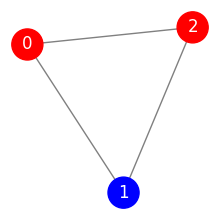
There are \(2^3\) colorings of the graph. In general there are \(2^n\) for an \(n\) node graph. The Max-cut problem can then be stated as that of finding the color assignment which maximizes the number of edges between nodes of a different color.

We can define the following cost function for solving the max-cut problem for a graph \(G\)

\[ \begin{equation*} C(G)= \frac{1}{2}\sum_{(i,j) \in E(G)} (1-z_i\,z_j)\,, \quad z_i,z_j \in \{-1,1\} \end{equation*} \]

Here \(z_i\) and \(z_j\) are variables representing the “colors” of each node and \(E(G)\) is the edge set of the graph. We can solve max-cut by finding a coloring of the graph that maximizes \(C(G)\)

Quantum Approximate Optimization Algorithm (QAOA)

General theory

Introduced in “A Quantum Approximate Optimization Algorithm” (found at https://arxiv.org/abs/1411.4028). The idea is to prepare a quantum state which encodes a solution to the max-cut problem. Measuring such a state will give us computational basis states (or bitstrings) which correspond to colorings of the graph.

QAOA is a variational algorithm, which is to say that a parameterized state is prepared, with the parameters varied to improve the solution. We will have \(2p\) parameters where \(p\) is our number of layers. In particular, the state prepared has the form

\[ | \psi ( \beta, \gamma ) \rangle = U_B ( \beta_{p-1} ) U_P ( \gamma_{p-1} ) ... U_B (\beta_0) U_P ( \gamma_0 ) | +\rangle ^{\otimes n} \]

where

\[ U_P ( \gamma_i) = e^{i \gamma_i H_P} \quad \& \quad U_B( \beta_i ) = e^{i \beta_i H_B} \]

We refer to \(H_{P} \equiv H_{P(G)}\) as the problem Hamiltonian. This Hamiltonian essentially encodes the connectivity of the graph in the max-cut problem.

\[ \begin{equation*} H_{P(G)} = \frac{1}{2}\sum_{(i, \,j) \in E(G)} (I-Z_i \,Z_j) \end{equation*} \]

Here there is an implicit tensor product. We use the notation \(Z_i \, Z_j \equiv Z_i \otimes Z_j\). Note also the resemblance between \(H_{P(G)}\) and our classical cost function \(C(G)\).

The rule for constructing this problem Hamiltonian is that we include a \(Z_i\, Z_j\) term for every edge \((i, j)\) in the graph. The section below shows how this Hamiltonian looks for a specific graph.

The \(H_B\) operator is called the mixer Hamiltonian. This operator is just a sum of Pauli \(X\) operators with one non-identity term on each qubit.

\[ \begin{equation*} H_B = \sum_i X_i \end{equation*} \]

Here we use the the convention that \(X_i\) means a Pauli \(X\) operator will be applied to the “ith” qubit and the identity operator will be applied to all other qubits in the circuit. Importantly, this mixer Hamiltonian does not commute with \(H_P\). This fact turns out to be important as it will allow us properly explore our solution space.

Example: cost and mixer Hamiltonian for a three node graph

Let us look again the three node graph we used in introducing the max-cut problem

plt.figure(figsize=(2, 2))
nx.draw(
    G,
    node_color=["red", "blue", "red"],
    font_size=12,
    font_color="white",
    node_size=500,
    edge_color="gray",
    with_labels=True,
)
plt.show()

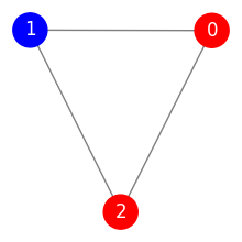
For the simple three node graph above the problem Hamiltonian is

\[ H_{P(G)} = \frac{3}{2} I - \frac{1}{2} \Big[ ( Z \otimes Z \otimes I ) + ( Z \otimes I \otimes Z ) + ( I \otimes Z \otimes Z ) \Big] \]

where you will notice that there is a \( Z \otimes Z\) acting between each node which is connected by an edge. The mixer Hamiltonian has the form

\[ H_B = ( X \otimes I \otimes I ) + ( I \otimes X \otimes I ) + ( I \otimes I \otimes X ) \]

Here there is an \(X\) operator acting on each node. The form of this operator is independent of the graph connectivity.

Building the program

To start off with, we will need to construct a QAOA circuit for a particular graph and number of layers (\(p\)). Our circuit for QAOA is constructed by alternating the cost layer (\(U_P\)) and mixer layer (\(U_B\)) \(p\) times for different parameters. The cost layer is defined by evolving the commuting Hamiltonian \(H_{P(G)}\). We can realize this with a layer of ZZPhase gates. For the mixer layer we are evolving the \(X\)-type Hamiltonian \(H_B\). We can realize the evolution with a layer of Rx gates.

\[\begin{split} \mathrm{Rx}(\beta)= \begin{pmatrix} \cos(\frac{ \beta}{2}) & -i\sin(\frac{ \beta}{2}) \\ -i\sin(\frac{ \beta}{2}) & \cos(\frac{ \beta}{2}) \end{pmatrix}\,, \qquad \mathrm{ZZPhase}(\gamma)= \exp(\frac{- i \gamma}{2}\big(Z \otimes Z \big))= \begin{pmatrix} e^{\frac{-i \gamma}{2}} & 0 & 0 & 0 \\ 0 & e^{\frac{i \gamma}{2}} & 0 & 0 \\ 0 & 0 & e^{\frac{i \gamma}{2}} & 0 \\ 0 & 0 & 0 & e^{\frac{-i \gamma}{2}} \end{pmatrix}\end{split}\]

We will define a Python function which will construct a Guppy program implementing QAOA for an \(n\) node graph. First we create the uniform superposition state \(|+\rangle^{\otimes n}\) and then alternate cost and mixer layers as described above.

The graph topology and the number of layers \(p\) are fixed at compile time (loaded with comptime expressions), but the cost and mixer angles are passed as runtime arguments: qaoa_instance takes two array[float, p] arguments. Because the angles are runtime arguments, the program can be compiled once and then re-run with different angle values — exactly what the variational optimization loop below needs.

from guppylang import guppy
from guppylang.std.quantum import qubit, h, rx
from guppylang.std.qsystem.helios import zz_phase
from guppylang.std.builtins import array
from guppylang.std.angles import pi
from guppylang.defs import GuppyFunctionDefinition


def build_qaoa_instance(graph: nx.Graph, n_layers: int) -> GuppyFunctionDefinition:
    edges = list(graph.edges)
    n_qubits = graph.number_of_nodes()

    @guppy
    def qaoa_instance(
        cost_angles: array[float, n_layers],
        mixer_angles: array[float, n_layers],
    ) -> array[qubit, n_qubits]:
        qs = array(qubit() for _ in range(n_qubits))
        n = len(qs)

        for i in range(n):
            h(qs[i])

        for layer in range(n_layers):
            # Add cost layer
            for i, j in edges:
                zz_phase(qs[i], qs[j], -cost_angles[layer] * pi / 2)

            # Add mixer layer
            for i in range(n):
                rx(qs[i], mixer_angles[layer] * pi)

        return qs

    return qaoa_instance

Calculating expectation values

We also need to extract our energy expectation values from a QsysResult object after our circuit is processed by the Selene simulator. We do this with the energy_from_result function below. Note that the fact that the max-cut problem Hamiltonian \(H_P\) contains only commuting terms means that we do not need to calculate our energy expectation using multiple measurement circuits.

from hugr.qsystem.result import QsysResult


def energy_from_result(graph: nx.Graph, result: QsysResult, n_shots: int) -> float:
    energy = 0.0
    dist = result.register_counts()["c"]
    for i, j in graph.edges:
        for meas, count in dist.items():
            prob = count / n_shots
            energy += (int(meas[i]) ^ int(meas[j])) * prob

    return energy

Now let’s define helpers for executing and scoring QAOA parameter values.

Because the cost and mixer angles are runtime arguments, we compile the program once and re-run it for every parameter set. build_qaoa_program defines a main entrypoint that takes the angles as arguments and returns a built EmulatorInstance. run_qaoa_circuit executes that instance for specific angle values by passing them to .run(...), and eval_qaoa_energy turns the result into the scalar energy needed by the classical optimizer.

The p_value argument defines the number of cost/mixer layers in the QAOA program.

import numpy as np
from guppylang.std.quantum import measure_array, collect_measurements
from guppylang.std.builtins import output
from guppylang.emulator import EmulatorInstance
from numpy.typing import NDArray


def build_qaoa_program(
    graph: nx.Graph,
    p_value: int,
    seed: int,
    shots: int,
) -> EmulatorInstance:
    qaoa_instance: GuppyFunctionDefinition = build_qaoa_instance(
        graph=graph,
        n_layers=p_value,
    )

    @guppy
    def main(
        cost_angles: array[float, p_value],
        mixer_angles: array[float, p_value],
    ) -> None:
        qaoa_qubits = qaoa_instance(cost_angles, mixer_angles)
        output("c", collect_measurements(measure_array(qaoa_qubits)))

    # Compiled and built once; reused for every parameter set via `.run(...)`.
    return (
        main.emulator(n_qubits=graph.number_of_nodes())
        .with_shots(shots)
        .with_seed(seed)
    )


def run_qaoa_circuit(
    program: EmulatorInstance,
    cost_angles: NDArray[np.float64],
    mixer_angles: NDArray[np.float64],
) -> QsysResult:
    return program.run(
        cost_angles=[float(x) for x in cost_angles],
        mixer_angles=[float(x) for x in mixer_angles],
    )


def eval_qaoa_energy(
    program: EmulatorInstance,
    cost_angles: NDArray[np.float64],
    mixer_angles: NDArray[np.float64],
    graph: nx.Graph,
    shots: int,
) -> float:
    qaoa_result = run_qaoa_circuit(program, cost_angles, mixer_angles)
    return energy_from_result(graph, qaoa_result, shots)

Setting up the variational loop

Now that we have the eval_qaoa_energy function which does a single “forward pass” of our algorithm, we can use a classical optimizer to find a set of parameters which maximizes the energy expectation value.

To accomplish this, we define a SciPy objective function that accepts a single parameter vector, splits it into QAOA cost and mixer coefficients, evaluates the Guppy program for those coefficients, and returns the negative energy. Minimizing the negative energy is equivalent to maximizing the max-cut energy.

Now we can put all of this machinery together in a solve_max_cut_instance function which, given a graph, attempts to solve the max-cut problem using this variational method. After the optimizer finishes, we run one final QAOA forward pass with the best parameters and use that QsysResult for validation and plotting.

Our function takes the following arguments:

• graph: A networkx graph for which we want to solve the max-cut problem.

• max_optimizer_iterations: The maximum number of objective evaluations in the SciPy optimizer.

• p_value: The number of alternating cost/mixer layers in our QAOA program.

• n_shots: The number of Guppy program executions for each expectation value calculation.

• seed: A seed for the random number generator so the initial parameters and emulator executions are reproducible.

The optimized values below are dimensionless coefficients of Guppy angle constants: the cost layer applies -cost_angle * pi / 2, and the mixer layer applies mixer_angle * pi. The optimizer works directly with these real-valued coefficients.

from scipy.optimize import OptimizeResult, minimize


def pack_qaoa_params(
    cost_angles: NDArray[np.float64], mixer_angles: NDArray[np.float64]
) -> NDArray[np.float64]:
    return np.concatenate((cost_angles, mixer_angles))


def split_qaoa_params(
    params: NDArray[np.float64], p_value: int
) -> tuple[NDArray[np.float64], NDArray[np.float64]]:
    return params[:p_value], params[p_value:]


def solve_max_cut_instance(
    graph: nx.Graph,
    max_optimizer_iterations: int,
    p_value: int,
    n_shots: int,
    seed: int,
) -> tuple[QsysResult, NDArray[np.float64], NDArray[np.float64], OptimizeResult]:
    rng = np.random.default_rng(seed)
    initial_params = pack_qaoa_params(
        cost_angles=rng.uniform(0, 2 * np.pi, size=p_value),
        mixer_angles=rng.uniform(0, 2 * np.pi, size=p_value),
    )

    # Compile and build the program once, then reuse it for every objective
    # evaluation by supplying the angles as runtime arguments.
    program = build_qaoa_program(
        graph=graph, p_value=p_value, seed=seed, shots=n_shots
    )

    def objective(params: NDArray[np.float64]) -> float:
        cost_angles, mixer_angles = split_qaoa_params(params, p_value)
        qaoa_energy = eval_qaoa_energy(
            program=program,
            cost_angles=cost_angles,
            mixer_angles=mixer_angles,
            graph=graph,
            shots=n_shots,
        )
        return -qaoa_energy

    optimizer_result = minimize(
        objective,
        initial_params,
        method="COBYLA",
        options={"maxiter": max_optimizer_iterations, "rhobeg": 0.5},
    )

    best_cost_angles, best_mixer_angles = split_qaoa_params(
        optimizer_result.x, p_value
    )
    best_result = run_qaoa_circuit(program, best_cost_angles, best_mixer_angles)

    return best_result, best_cost_angles, best_mixer_angles, optimizer_result

Solving max-cut for a graph with seven nodes

Now that we have all of the pieces ready, let’s test our QAOA implementation for a very simple graph.

We will graph where the correct answer for max-cut is very easy to verify manually.

max_cut_graph_edges = [(0, 1), (1, 2), (1, 3), (3, 4), (4, 5), (4, 6)]
n_nodes = 7

max_cut_graph = nx.Graph()
max_cut_graph.add_edges_from(max_cut_graph_edges)
pos = nx.kamada_kawai_layout(max_cut_graph)
nx.draw(
    max_cut_graph,
    pos=pos,
    labels={node: node for node in max_cut_graph.nodes()},
    font_size=12,
    font_color="white",
    node_size=500,
    edge_color="gray",
)

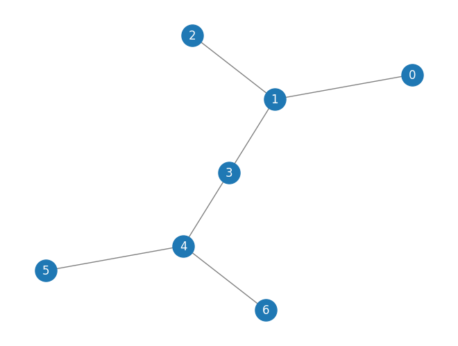
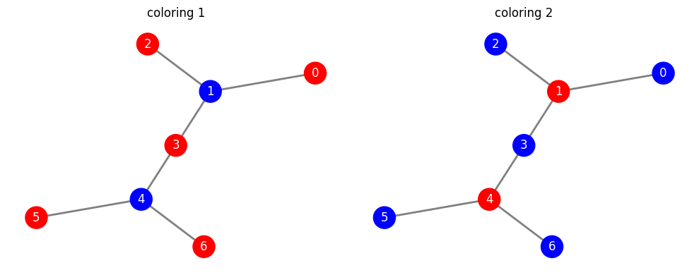
The solution for this graph is a simple alternating coloring which we can represent with the following pair of bitstrings. See the two graphs drawn at the end of this notebook. The bitstrings are the binary complement of one another.

We have chosen a sparse graph where it is easy to check the mx-cut solution by inspection. For this configuration, the solution is that nodes 1 and 4 are a different color to nodes 0, 2, 3, 5 and 6.

We can represent a coloring with a binary string where the “ith” entry in the string represents the color of node i. Therefore the expected solutions can be represented by the following two strings.

expected_result_strings = ["0100100", "1011011"]

Note that there are two colourings as all that matters is that we have partitioned the node indices into the sets \(S_0=\{0, 2, 3, 5, 6\}\) and \(S_1=\{1, 4\}\). If we have two colors e.g. red and blue, then we have the freedom to colour the nodes in \(S_0\) blue and \(S_1\) red or vice-versa.

Now we need a problem Hamiltionian which reflects the connectivity of our graph. Recall how the problem Hamiltonian is defined.

\[ \begin{equation*} H_{P(G)} = \frac{1}{2}\sum_{(i, \,j) \in E(G)} (I-Z_i \,Z_j) \end{equation*} \]

Four our seven vertex graph, the problem Hamiltonian is the following

\[ \begin{equation*} H_{P(G)} = 3 I_{(n=7)} -\frac{1}{2} \big[ Z_0 Z_1 + Z_1 Z_2 +Z_1 Z_3 +Z_3 Z_4 +Z_4 Z_5 +Z_4 Z_6 \big]\, . \end{equation*} \]

The form of the mixer Hamiltonian \(H_B\) depends only on the number of nodes in our graph. The evolution operator \(U_B\) can be implemented with a layer of Rx gates. See the build_qaoa_instance function.

n_shots = 2000
p_value = 3
random_seed = 12345
max_optimizer_iterations = 100

qaoa_result, cost_angles, mixer_angles, optimizer_result = solve_max_cut_instance(
    n_shots=n_shots,
    max_optimizer_iterations=max_optimizer_iterations,
    graph=max_cut_graph,
    seed=random_seed,
    p_value=p_value,  # Cost-mixer layers
)

optimized_energy = -float(optimizer_result.fun)
print(f"Optimizer status: {optimizer_result.message}")
print(f"Objective evaluations: {optimizer_result.nfev}")
print(f"Optimized energy: {optimized_energy:.4f}")
print(f"Cost angles: {np.round(cost_angles, 3)}")
print(f"Mixer angles: {np.round(mixer_angles, 3)}")

Optimizer status: Return from COBYLA because the trust region radius reaches its lower bound.
Objective evaluations: 77
Optimized energy: 5.0995
Cost angles: [1.736 2.63  4.751]
Mixer angles: [4.831 2.361 2.2  ]

Optimizer status note. COBYLA is a derivative-free trust-region optimizer. If it reports that the trust-region radius reached its lower bound, that is a normal termination condition: the local search radius has shrunk to the configured tolerance. If it reports that the maximum number of function evaluations was exceeded, the configured maxiter budget was exhausted.

The optimizer objective above maximizes the expected max-cut energy. This is related to, but not identical to, maximizing the probability of sampling one of the two exact optimal colorings.

Lets define a function that checks that the most frequent measurement outcomes correspond to the expected graph colorings.

def validate_qaoa_experiment(
    result: QsysResult, expected_colorings: list[str], n_shots: int
) -> float:
    counts_dict = result.register_counts()["c"]
    sorted_shots = counts_dict.most_common()
    most_common_states = [entry[0] for entry in sorted_shots[:2]]

    if set(most_common_states) != set(expected_colorings):
        raise ValueError(
            "The most frequently measured outcomes "
            f"{most_common_states} did not correspond to the expected graph coloring."
        )

    num_successful_shots = sum(entry[1] for entry in sorted_shots[:2])
    return num_successful_shots / n_shots

success_ratio = validate_qaoa_experiment(
    qaoa_result, expected_result_strings, n_shots
)
f"Success ratio: {success_ratio:.4f}"

'Success ratio: 0.4015'

The success ratio above counts only samples that land in the two optimal colorings. To compare it with the optimized energy objective, we can group all sampled bitstrings by their max-cut value.

from collections import Counter


def cut_value(bitstring: str, graph: nx.Graph) -> int:
    return sum(int(bitstring[i]) ^ int(bitstring[j]) for i, j in graph.edges)


def summarize_cut_distribution(
    result: QsysResult, graph: nx.Graph, optimal_colorings: list[str]
) -> None:
    counts = result.register_counts()["c"]
    total_shots = sum(counts.values())
    counts_by_cut = Counter()

    for bitstring, count in counts.items():
        counts_by_cut[cut_value(bitstring, graph)] += count

    expected_energy = sum(
        cut * count for cut, count in counts_by_cut.items()
    ) / total_shots
    optimal_probability = sum(
        counts.get(bitstring, 0) for bitstring in optimal_colorings
    ) / total_shots

    print(f"Expected energy from sampled distribution: {expected_energy:.4f}")
    print(f"Probability of optimal colorings: {optimal_probability:.4f}")
    print("Probability by cut value:")
    for cut, count in sorted(counts_by_cut.items()):
        print(f"  cut={cut}: {count / total_shots:.4f}")


summarize_cut_distribution(qaoa_result, max_cut_graph, expected_result_strings)

Expected energy from sampled distribution: 5.0995
Probability of optimal colorings: 0.4015
Probability by cut value:
  cut=1: 0.0005
  cut=2: 0.0175
  cut=3: 0.0425
  cut=4: 0.1625
  cut=5: 0.3755
  cut=6: 0.4015

Finally, we can plot the most common measurement outcomes. If we have done this correctly then the two most common measurement outcomes should correspond to the graph colorings which solve our instance of the max-cut problem

import matplotlib.pyplot as plt


def plot_max_cut_results(result: QsysResult, n_strings: int) -> None:
    """
    Plots Max-cut results in a barchart with the two most common bitstrings highlighted in green.
    """
    counts_dict = result.register_counts()["c"]
    sorted_shots = counts_dict.most_common()
    n_shots = sum(counts_dict.values())

    n_most_common_strings = sorted_shots[:n_strings]
    x_axis_values = [str(entry[0]) for entry in n_most_common_strings]  # basis states
    y_axis_values = [entry[1] for entry in n_most_common_strings]  # counts

    fig = plt.figure()
    ax = fig.add_axes([0, 0, 1.5, 1])
    color_list = ["green"] * 2 + (["orange"] * (len(x_axis_values) - 2))
    ax.bar(
        x=x_axis_values,
        height=y_axis_values,
        color=color_list,
    )
    ax.set_title(label="Max-cut Results")
    plt.ylim([0, 0.25 * n_shots])
    plt.xlabel("Basis State")
    plt.ylabel("Number of Shots")
    plt.show()


plot_max_cut_results(qaoa_result, n_strings=6)

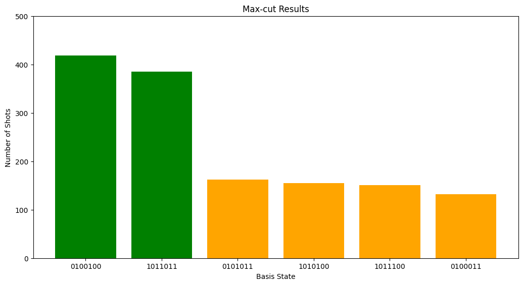
The two green bars correspond to the expected colorings of our seven vertex graph. These colorings are equivalent up to the swapping of blue and red nodes.

G = nx.Graph()
G.add_edges_from(max_cut_graph_edges)

H = nx.Graph()
H.add_edges_from(max_cut_graph_edges)

# Use same layout for both graphs
pos = nx.kamada_kawai_layout(G)

fig, axes = plt.subplots(1, 2, figsize=(10, 4))

# First coloring
nx.draw(
    G,
    pos=pos,
    ax=axes[0],
    with_labels=True,
    node_color=["red", "blue", "red", "red", "blue", "red", "red"],
    node_size=500,
    edge_color="gray",
    width=2,
    font_size=12,
    font_color="white",
)
axes[0].set_title("coloring 1")
axes[0].set_axis_off()

# Second coloring
nx.draw(
    H,
    pos=pos,
    ax=axes[1],
    with_labels=True,
    node_color=["blue", "red", "blue", "blue", "red", "blue", "blue"],
    node_size=500,
    edge_color="gray",
    width=2,
    font_size=12,
    font_color="white",
)
axes[1].set_title("coloring 2")
axes[1].set_axis_off()

plt.tight_layout()
plt.show()